multi-database
Martin Garlovsky
2021-01-26
Last updated: 2022-02-07
Checks: 7 0
Knit directory: virilisProteomics/
This reproducible R Markdown analysis was created with workflowr (version 1.6.2). The Checks tab describes the reproducibility checks that were applied when the results were created. The Past versions tab lists the development history.
Great! Since the R Markdown file has been committed to the Git repository, you know the exact version of the code that produced these results.
Great job! The global environment was empty. Objects defined in the global environment can affect the analysis in your R Markdown file in unknown ways. For reproduciblity it’s best to always run the code in an empty environment.
The command set.seed(20201210) was run prior to running the code in the R Markdown file. Setting a seed ensures that any results that rely on randomness, e.g. subsampling or permutations, are reproducible.
Great job! Recording the operating system, R version, and package versions is critical for reproducibility.
Nice! There were no cached chunks for this analysis, so you can be confident that you successfully produced the results during this run.
Great job! Using relative paths to the files within your workflowr project makes it easier to run your code on other machines.
Great! You are using Git for version control. Tracking code development and connecting the code version to the results is critical for reproducibility.
The results in this page were generated with repository version 60b9ff5. See the Past versions tab to see a history of the changes made to the R Markdown and HTML files.
Note that you need to be careful to ensure that all relevant files for the analysis have been committed to Git prior to generating the results (you can use wflow_publish or wflow_git_commit). workflowr only checks the R Markdown file, but you know if there are other scripts or data files that it depends on. Below is the status of the Git repository when the results were generated:
Ignored files:
    Ignored:    .DS_Store
    Ignored:    .RData
    Ignored:    .Rhistory
    Ignored:    .Rproj.user/
    Ignored:    analysis/.DS_Store
    Ignored:    analysis/.Rhistory
    Ignored:    code/.DS_Store
    Ignored:    data/.DS_Store
    Ignored:    output/.DS_Store

Untracked files:
    Untracked:  .Rapp.history
    Untracked:  TrialDataFirstLook.R
    Untracked:  alignment_dotplot_dark_AN.png
    Untracked:  code/.ipynb_checkpoints/
    Untracked:  code/find_seq.py
    Untracked:  comparisons/
    Untracked:  data/ABetal.2020/
    Untracked:  data/Dvir_stringtie_transcripts_lengths.txt
    Untracked:  data/FlyBase_GO_STEP.txt
    Untracked:  data/Garlovsky_etal_Dmon_MaxQuant_ParkerID.csv
    Untracked:  data/Orthogroups.tsv
    Untracked:  data/PEAKS/
    Untracked:  data/ProteomeDiscoverer/
    Untracked:  data/RNASeq_data/
    Untracked:  data/mRNA_abundances/
    Untracked:  data/melanogaster/
    Untracked:  data/reciprocal_orths.csv
    Untracked:  data/signal_peptides/
    Untracked:  data/vir_annotation.rds
    Untracked:  data/virilis_Accession2FBgn_uniprot.csv
    Untracked:  data/virilis_male_AG_SFP_EB_genes.txt
    Untracked:  data/virilis_molecular_evolution_results/
    Untracked:  output/ClueGOlists/
    Untracked:  output/combined_database.csv
    Untracked:  plots/

Unstaged changes:
    Deleted:    analysis/data-exploration.Rmd
    Deleted:    analysis/differential-abundance.Rmd
    Modified:   code/mRNA_integration_analysis.ipynb
Note that any generated files, e.g. HTML, png, CSS, etc., are not included in this status report because it is ok for generated content to have uncommitted changes.
These are the previous versions of the repository in which changes were made to the R Markdown (analysis/multi-database.Rmd) and HTML (docs/multi-database.html) files. If you’ve configured a remote Git repository (see ?wflow_git_remote), click on the hyperlinks in the table below to view the files as they were in that past version.
| File | Version | Author | Date | Message |
|---|---|---|---|---|
| Rmd | 60b9ff5 | MartinGarlovsky | 2022-02-07 | wflow_publish(“analysis/multi-database.Rmd”) |
| html | f28e7a0 | MartinGarlovsky | 2022-02-07 | Build site. |
| Rmd | e7a1534 | MartinGarlovsky | 2022-02-07 | complete analysis biorXiv |
| html | 25c4f65 | MartinGarlovsky | 2022-01-19 | Build site. |
| Rmd | fb66329 | MartinGarlovsky | 2022-01-19 | wflow_publish(“analysis/multi-database.Rmd”) |
| html | db9953e | MartinGarlovsky | 2022-01-19 | Build site. |
| Rmd | ca4efd5 | MartinGarlovsky | 2022-01-19 | wflow_publish(“analysis/multi-database.Rmd”) |
| html | 4132227 | MartinGarlovsky | 2021-12-16 | Build site. |
| Rmd | 427c70d | MartinGarlovsky | 2021-12-16 | update analysis |
| html | 7430abe | MartinGarlovsky | 2021-12-15 | Build site. |
| Rmd | 34bb48b | MartinGarlovsky | 2021-12-15 | analysis update |
Introduction
The following analyses are the results of a 16-plex TMT labelling proteomics experiment. Flies were flash frozen in liquid nitrogen within ~30 seconds after copulation ended and stored at -80ºC. Later, female flies were thawed and the lower reproductive tract dissected with fine forceps in a drop of 1X PBS, rinsed in a second drop, and then added to a pool (n = ) of XXX kept on ice. Samples were shipped on dry ice to the Cambridge Core Proteomics Facility, UK, for LC-MS/MS. Resulting .raw files were processed in Proteome Discoverer using each species’ proteome.
Load packages
library(tidyverse)
library(tidybayes)
library(ggrepel)
library(ComplexHeatmap)
library(grid)
library(UpSetR)
library(RColorBrewer)
library(eulerr)
library(edgeR)
library(kableExtra)
library(DT)

# colour palettes

# colourblind friendly palette
cbPalette <- c("#999999", "#E69F00", "#56B4E9", "#009E73", "#F0E442", "#CC79A7", "#D55E00", "#0072B2", "#CC79A7")

# viridis palettes
v.pal <- viridis::viridis(n = 3, direction = -1)
m.pal <- viridis::magma(n = 5, direction = -1)
c.pal <- viridis::inferno(n = 7)

# nice tables
my_data_table <- function(df){
  datatable(
    df, rownames = FALSE,
    autoHideNavigation = TRUE,
    extensions = c("Scroller",  "Buttons"),
    options = list(
      dom = 'Bfrtip',
      deferRender = TRUE,
      scrollX = TRUE, scrollY = 400,
      scrollCollapse = TRUE,
      buttons =
        list('csv', list(
          extend = 'pdf',
          pageSize = 'A4',
          orientation = 'landscape',
          filename = 'Dpseudo_respiration')),
      pageLength = 50
    )
  )
}
Tree
Phylogenetic relationship between the three species used in our study.
library(ape)
tree <- read.tree(text = "((D. nov, D. ame),D. vir);")
#pdf('plots/tree.pdf', height = 3, width = 4)
plot(tree, type = 'cladogram', edge.width = 2, label.offset = .1)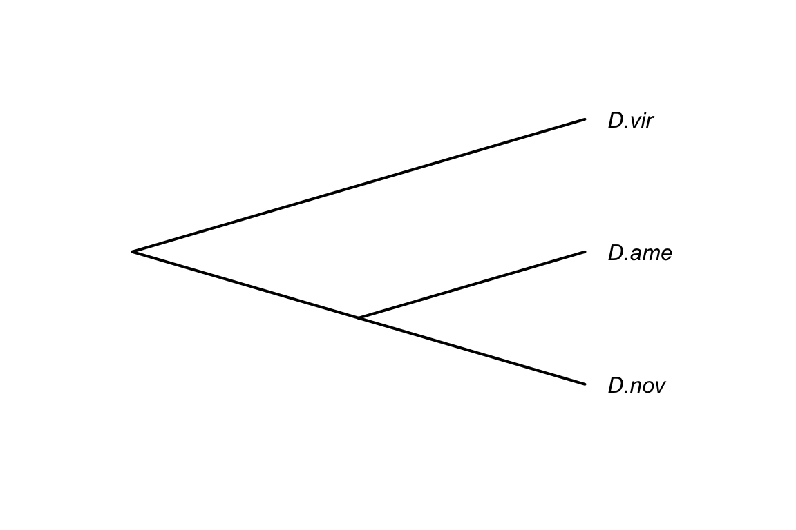
| Version | Author | Date |
|---|---|---|
| 7430abe | MartinGarlovsky | 2021-12-15 |
#dev.off()Load data
Protein abundance data exported from Proteome Discoverer using each species search
Trinotate gene annotations for D. virilis and .gff
virilis group accessory gland, ejaculatory bulb and seminal fluid protein genes
List of D. melanogaster sperm protein orthologs from Wasborough et al. (2009), comprising 1108 proteins, combined with the DmSP1
List of putative D. melanogaster Sfps identified by Wigby et al. (2020). Phil. trans. B
Orthology table between D. melanogaster and D. virilis FBgns
Male accessory gland or ejaculatory bulb biased genes and putative SFPs from Ahmed-Braimah et al. (2017) G3
Female reproductive tract biased genes and postmating response genes from Ahmed-Braimah et al. (2021) MBE
Pairwise dN/dS results also from Ahmed-Braimah et al. (2021) MBE
Signal peptide predictions for each species from Phobius and SignalP-5.0
Gene ontology (GO) information for all D. virilis genes from FlyBase.org
Orthofinder orthogroups results for reciprocal orthology between species for all proteins
# load Proteome Discoverer data searched against each species
ame_Dat <- read.delim('data/ProteomeDiscoverer/P790_Garlovsky_newdb_22012021/P790_ane_220121_Proteins.txt') %>% filter(!str_detect(Accession, 'cRAP'))
nov_Dat <- read.delim('data/ProteomeDiscoverer/P790_Garlovsky_newdb_22012021/P790_nov_220121_Proteins.txt') %>% filter(!str_detect(Accession, 'cRAP'))
vir_Dat <- read.delim('data/ProteomeDiscoverer/P790_Garlovsky_newdb_22012021/P790_vit_220121_Proteins.txt') %>% filter(!str_detect(Accession, 'cRAP'))

# replace colnames
old.names <- c('126', '127N', '127C', '128N', '128C', '129N', '129C', '130N', '130C', '131N', '131C', '132N', '132C', '133N', '133C', '134N')
new.names <- c('AM1', 'AM2', 'AM3', 'AV1', 'AV2', 'NM1', 'NM2', 'NM3', 'NV1', 'NV2', 'VM1', 'VM2', 'VM3', 'VV1', 'VV2', 'VV3')

colnames(ame_Dat) <- stringi::stri_replace_all_fixed(colnames(ame_Dat), pattern = old.names,
                                                     replacement = new.names, vectorize_all = FALSE)

colnames(nov_Dat) <- stringi::stri_replace_all_fixed(colnames(nov_Dat), pattern = old.names,
                                                     replacement = new.names, vectorize_all = FALSE)

colnames(vir_Dat) <- stringi::stri_replace_all_fixed(colnames(vir_Dat), pattern = old.names,
                                                     replacement = new.names, vectorize_all = FALSE)

# compare abundances between runs
bind_rows(
  ame_Dat %>%
    select(starts_with('Abun')) %>%
    pivot_longer(1:16) %>%
    mutate(name = str_remove_all(name, 'Abundances.Grouped.F1.'),
           species = str_sub(name, 1, 1),
           mating = str_sub(name, 2, 2),
           condition = str_sub(name, 1, 2),
           mapping = 'ame'),
  nov_Dat %>%
    select(starts_with('Abun')) %>%
    pivot_longer(1:16) %>%
    mutate(name = str_remove_all(name, 'Abundances.Grouped.F1.'),
           species = str_sub(name, 1, 1),
           mating = str_sub(name, 2, 2),
           condition = str_sub(name, 1, 2),
           mapping = 'nov'),
  vir_Dat %>%
    select(starts_with('Abun')) %>%
    pivot_longer(1:16) %>%
    mutate(name = str_remove_all(name, 'Abundances.Grouped.F1.'),
           species = str_sub(name, 1, 1),
           mating = str_sub(name, 2, 2),
           condition = str_sub(name, 1, 2),
           mapping = 'vir')) %>%
  ggplot(aes(x = name, y = log2(value + 1))) +
  geom_boxplot(aes(fill = mapping), notch = TRUE, outlier.shape = 1) +
  scale_fill_manual(values = viridis::viridis(n = 3),
                    name = "Database:",
                    labels = c(expression(italic('D. ame')),
                               expression(italic('D. nov')),
                               expression(italic('D. vir')))) +
  labs(y = 'log2(Abundance + 1)') +
  theme_bw() +
  theme(legend.position = 'bottom',
        legend.title = element_blank(),
        axis.title.x = element_blank()) +
  NULL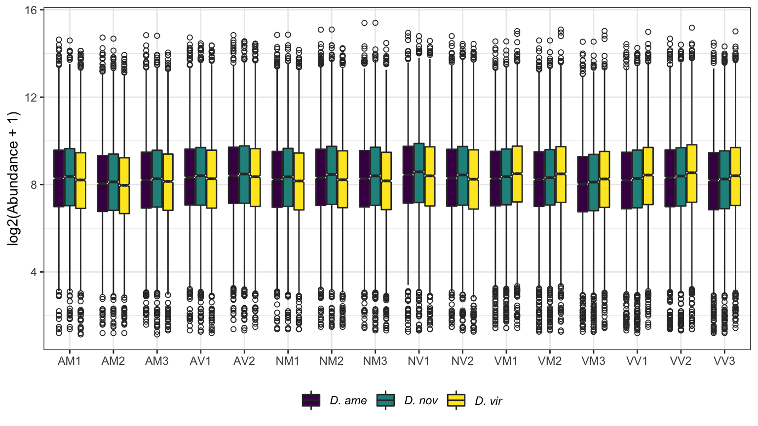
# now remove start of colname string for abundances
colnames(ame_Dat) <- gsub('Abundances.Grouped.F1.', '', colnames(ame_Dat))
colnames(nov_Dat) <- gsub('Abundances.Grouped.F1.', '', colnames(nov_Dat))
colnames(vir_Dat) <- gsub('Abundances.Grouped.F1.', '', colnames(vir_Dat))

# remove info from accession
ame_Dat$Accession <- gsub(' .*', '', x = ame_Dat$Accession)
nov_Dat$Accession <- gsub(' .*', '', x = nov_Dat$Accession)
vir_Dat$Accession <- gsub(' .*', '', x = vir_Dat$Accession)

### FlyBase gene IDS
vir_ids <- inner_join(
  # MSTRG to FBtr
  read.delim('data/virilis_molecular_evolution_results/PacBio_virilis_Trinotate_report.xls') %>%
  select(X.gene_id, transcript_id, prot_id, dvir.proteins.fasta_BLASTX) %>%
  mutate(FBtr = gsub('\\^.*', '', x = dvir.proteins.fasta_BLASTX)) %>%
  select(-dvir.proteins.fasta_BLASTX),
  # FBgn to FBtr table
  read.delim('data/virilis_molecular_evolution_results/gffread_annotated_transcripts.gene_trans_map',
             header = FALSE) %>%
  dplyr::rename(FBgn = V1,
                FBtr = V2),
  by = 'FBtr')

# virilis group AG/SFP/EB biased genes
Dvir_SFPs <- read.delim('data/virilis_male_AG_SFP_EB_genes.txt', header = FALSE) %>%
  dplyr::rename(bias = V1,
                FBgn = V2)

# Dmel sperm proteome orthologs
sperm_mel <- inner_join(
  # Dmel Sperm proteome II (Wasbrough et al. 2010 J. Prot.)
  read.csv('data/melanogaster/DmSPii_Supp.Table3.csv'),
  # melanogaster orthologs
  read.table(file = "data/melanogaster/mel_orths.txt", header = T),
  by = c('Gene.Symbol' = 'mel_GeneSymbol')) %>%
  distinct(FBgn_ID, .keep_all = TRUE) %>%
  select(FBgn_v = FBgn_ID, Gene.Name, Gene.Symbol, mel_Arm) %>%
  left_join(vir_ids, by = c('FBgn_v' = 'FBgn'))

# Dmel SFP orthologs
wigbySFP <- inner_join(
  # List of SFPs (Wigby et al. 2020 Phil. Trans. B.)
  read.csv('data/melanogaster/dmel_SFPs_wigby_etal2020.csv') %>%
  filter(category == 'highconf'),
  # melanogaster orthologs
  read.table(file = "data/melanogaster/mel_orths.txt", header = T),
  by = c('FBgn' = 'mel_FBgn_ID')) %>%
  select(FBgn = FBgn_ID, FBgn_mel = FBgn, Symbol) %>%
  left_join(vir_ids, by = c('FBgn')) %>%
  distinct(FBgn, .keep_all = TRUE)

# Ahmed-Braimah et al. 2020 MBE data
# virilis gene FBgns FRT biased genes
FRTbiased <- readxl::read_excel('data/ABetal.2020/File_S1.xlsx')
# virilis gene FBgns changing in expression after mating
virilisPMDE <- readxl::read_excel('data/ABetal.2020/File_S3.xlsx')

# pairwise Ka.Ks values
kaks_results <- read.delim('data/virilis_molecular_evolution_results/KaKs.ALL.results.txt') %>%
  left_join(vir_ids, by = c('FBtr_ID' = 'FBtr'))

# FlyBase GO terms
flybase_GO <- read.delim('data/FlyBase_GO_STEP.txt') %>%
  dplyr::rename(FBgn = X.SUBMITTED.ID) %>%
  # merge Dmel orthologs and IDs
  left_join(read.table(file = "data/melanogaster/mel_orths.txt", header = T),
            by = c('FBgn' = 'FBgn_ID')) %>%
  distinct(FBgn, .keep_all = TRUE)

# OrthoFinder orthogroups output
orthogroups <- read_tsv('data/Orthogroups.tsv')
colnames(orthogroups) <- c('Orthogroup', 'ame', 'nov', 'vir')
Load Orthofinder results
We used Orthofinder to identify reciprocal 1:1:1 orthologs (i.e. ‘Orthogroups’) between each species. We used each species .pep/fasta sequences as input with default settings. Here, we parse the results and compile data matching orthogroups to the corresponding species-specific abundance data.
# omit NAs as we are only interseted in reciprocal 1:1:1 between all species
orth2 <- na.omit(orthogroups)

ame_group <- str_split(gsub(' ', '', x = orth2$ame), pattern = ',')
nov_group <- str_split(gsub(' ', '', x = orth2$nov), pattern = ',')
vir_group <- str_split(gsub(' ', '', x = orth2$vir), pattern = ',')

names(ame_group) <- orth2$Orthogroup
names(nov_group) <- orth2$Orthogroup
names(vir_group) <- orth2$Orthogroup

orthogroup_long <- bind_rows(
  reshape2::melt(ame_group) %>% mutate(species = 'ame'),
  reshape2::melt(nov_group) %>% mutate(species = 'nov'),
  reshape2::melt(vir_group) %>% mutate(species = 'vir')) %>%
  dplyr::rename(Accession = value, Orthogroup = L1)

ortho_ame <- ame_Dat %>% left_join(orthogroup_long %>% filter(species == 'ame') %>% select(Orthogroup, Accession)) %>% drop_na(Orthogroup)
ortho_nov <- nov_Dat %>% left_join(orthogroup_long %>% filter(species == 'nov') %>% select(Orthogroup, Accession)) %>% drop_na(Orthogroup)
ortho_vir <- vir_Dat %>% left_join(orthogroup_long %>% filter(species == 'vir') %>% select(Orthogroup, Accession)) %>% drop_na(Orthogroup)

# upset(fromList(list(
#   Dame = ortho_ame$Orthogroup,
#   Dnov = ortho_nov$Orthogroup,
#   Dvir = ortho_vir$Orthogroup)))

# plot overlap
plot(venn(c('Dame' = 345, 'Dnov' = 91, 'Dvir' = 94,
            'Dame&Dnov' = 288, 'Dame&Dvir' = 199, 'Dnov&Dvir' = 229,
            'Dame&Dnov&Dvir' = 2704)),
     quantities = TRUE,
     fills = list(fill = viridis::viridis(n = 3), alpha = .5))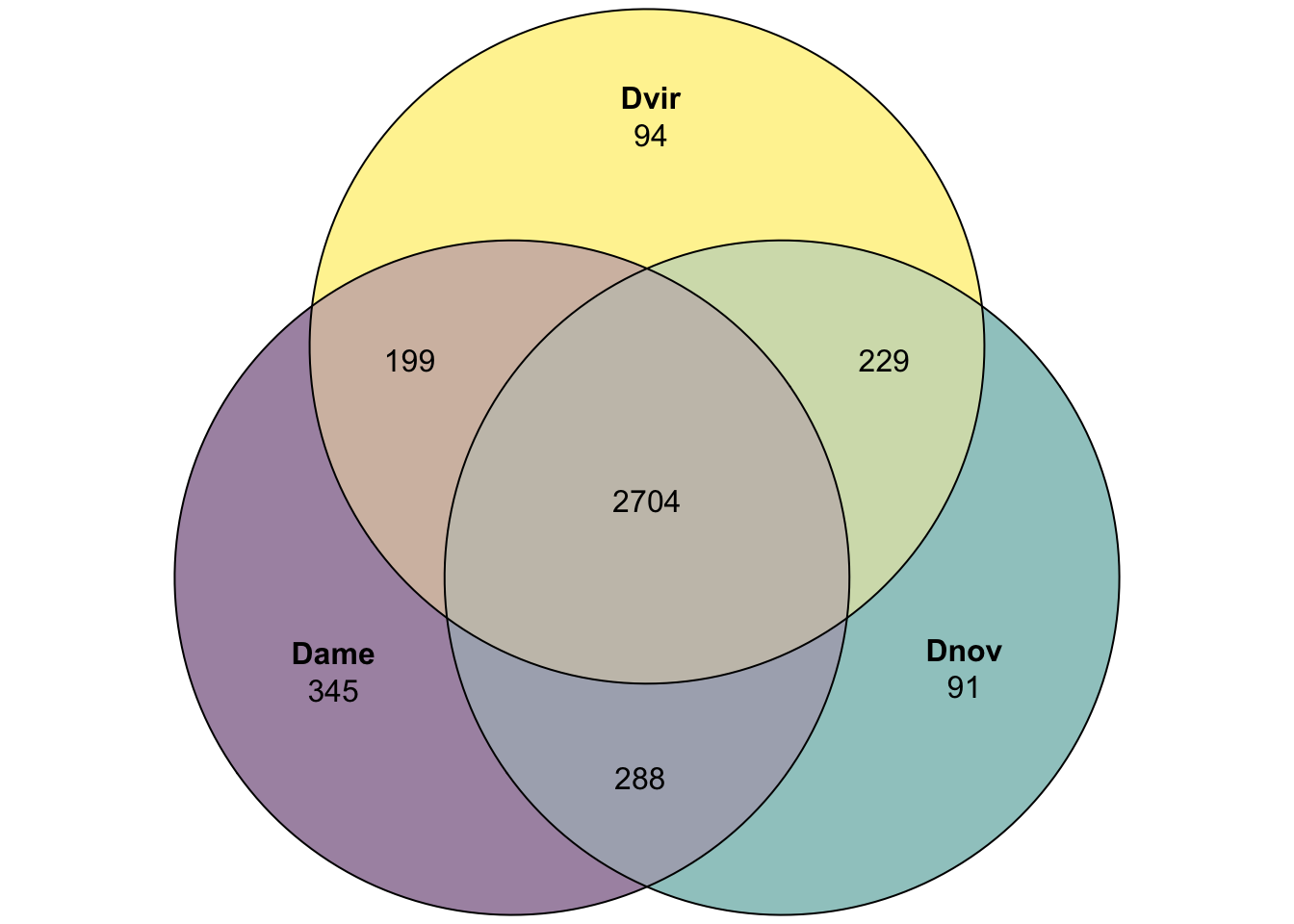
| Version | Author | Date |
|---|---|---|
| f28e7a0 | MartinGarlovsky | 2022-02-07 |
mdb <- ortho_ame %>%
  inner_join(ortho_nov, by = 'Orthogroup', suffix = c('_ame', '_nov')) %>%
  inner_join(ortho_vir, by = 'Orthogroup') %>%
  distinct(Orthogroup, .keep_all = TRUE)

colnames(mdb)[100:148] <- paste0(colnames(mdb)[100:148], '_vir')

recip_dat <- mdb %>%
  left_join(vir_ids %>% select(prot_id, FBtr, FBgn),
            by = c('Accession_vir' = 'prot_id'))

# # write file for dryad
# write_csv(recip_dat, 'output/combined_database.csv')
Load signal peptides predictions
We submitted each species proteome to Phobius and ran SignalP-5.0 locally to identify predicted signal peptide sequences and then combined the results.
# Phobius results
phob_ame <- read.csv('data/signal_peptides/PHOBIUS-predictions_stringtie_ame.csv') %>%
  dplyr::rename(ID = SEQENCE.ID)
phob_nov <- read.csv('data/signal_peptides/PHOBIUS-predictions_stringtie_nov.csv') %>%
  dplyr::rename(ID = SEQENCE.ID)
phob_vir <- read.csv('data/signal_peptides/PHOBIUS-predictions_stringtie_vir.csv') %>%
  dplyr::rename(ID = SEQENCE.ID)

# SigP results
sigP_ame <- read.csv('data/signal_peptides/ame_stringtie_short_summary.csv') %>%
  dplyr::rename(ID = X..ID)
sigP_nov <- read.csv('data/signal_peptides/nov_stringtie_short_summary.csv') %>%
  dplyr::rename(ID = X..ID)
sigP_vir <- read.csv('data/signal_peptides/vir_stringtie_short_summary.csv') %>%
  dplyr::rename(ID = X..ID)

# overlap between methods
# upset(fromList(list(
#   Phobius = phob_vir %>%
#     filter(SP == 'Y' & ID %in% vir_Dat$Accession) %>% pull(ID),
#   SignalP = sigP_vir %>%
#     filter(Prediction == 'SP(Sec/SPI)' & ID %in% vir_Dat$Accession) %>% pull(ID))))

# combine results
signal_peps_ame <- combine(phob_ame %>%
                             filter(SP == 'Y' & ID %in% ame_Dat$Accession) %>%
                             select(ID),
                           sigP_ame %>%
                             filter(Prediction == 'SP(Sec/SPI)' & ID %in% ame_Dat$Accession) %>%
                             select(ID)) %>% distinct()

signal_peps_nov <- combine(phob_nov %>%
                             filter(SP == 'Y' & ID %in% nov_Dat$Accession) %>%
                             select(ID),
                           sigP_nov %>%
                             filter(Prediction == 'SP(Sec/SPI)' & ID %in% nov_Dat$Accession) %>%
                             select(ID)) %>% distinct()

signal_peps_vir <- combine(phob_vir %>%
                             filter(SP == 'Y' & ID %in% vir_Dat$Accession) %>%
                             select(ID),
                           sigP_vir %>%
                             filter(Prediction == 'SP(Sec/SPI)' & ID %in% vir_Dat$Accession) %>%
                             select(ID)) %>% distinct()

ame_sig <- signal_peps_ame %>%
  left_join(orthogroup_long, by = c('ID' = 'Accession'))

nov_sig <- signal_peps_nov %>%
  left_join(orthogroup_long, by = c('ID' = 'Accession'))

vir_sig <- signal_peps_vir %>%
  left_join(orthogroup_long, by = c('ID' = 'Accession')) %>%
  left_join(vir_ids, by = c('ID' = 'prot_id'))

# #overlap between species
# upset(fromList(list(
#   Dame = ame_sig$Orthogroup,
#   Dnov = nov_sig$Orthogroup,
#   Dvir = vir_sig$Orthogroup)))

#pdf('plots/SignalPeps_overlap.pdf', height = 4, width = 4)
plot(venn(c('Dame' = 44, "Dnov" = 71, "Dvir" = 73,
                   'Dame&Dnov' = 95, 'Dame&Dvir' = 82, 'Dnov&Dvir' = 145,
                   'Dame&Dnov&Dvir' = 422)),
     quantities = TRUE,
     fills = list(fill = viridis::viridis(n = 3), alpha = .5))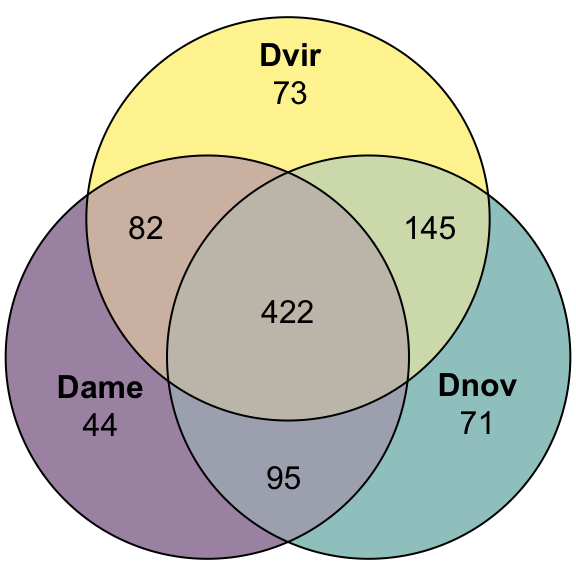
| Version | Author | Date |
|---|---|---|
| f28e7a0 | MartinGarlovsky | 2022-02-07 |
#dev.off()Differential abundance analysis
We performed differential abundance analysis between mated and virgin samples for each species, and between species, using each species database. We considered proteins as differentially abundant based on an adjusted p-value < 0.05 and logFC > |1|.
Single species database analysis
Identifying ejaculate candidates
# filter data for two unique peptides
ame_abund <- ame_Dat %>%
  dplyr::select(Accession, unique.p = Number.of.Unique.Peptides, 16:31) %>%
  filter(unique.p >= 2) %>%
  mutate(across(3:18, ~replace_na(.x, 0)))

nov_abund <- nov_Dat %>%
  dplyr::select(Accession, unique.p = Number.of.Unique.Peptides, 16:31) %>%
  filter(unique.p >= 2) %>%
  mutate(across(3:18, ~replace_na(.x, 0)))

vir_abund <- vir_Dat %>%
  dplyr::select(Accession, unique.p = Number.of.Unique.Peptides, 16:31) %>%
  filter(unique.p >= 2) %>%
  mutate(across(3:18, ~replace_na(.x, 0)))

# get sample info - same for all db's
sampInfo = data.frame(condition = str_sub(colnames(ame_abund[-c(1:2)]), 1, 2),
                      Replicate = str_sub(colnames(ame_abund[-c(1:2)]), 3, 3))

# make design matrix to test diffs between groups
design <- model.matrix(~0 + sampInfo$condition)
colnames(design) <- unique(sampInfo$condition)
rownames(design) <- sampInfo$Replicate

# make contrasts - higher values = higher in mated
cont.matrix <- makeContrasts(M.a.V = AM - AV,
                             M.n.V = NM - NV,
                             M.v.V = VM - VV,
                             levels = design)

# create DGElist and fit model
dge_ame <- DGEList(counts = ame_abund[, -c(1:2)], genes = ame_abund$Accession, group = sampInfo$condition)
dge_nov <- DGEList(counts = nov_abund[, -c(1:2)], genes = nov_abund$Accession, group = sampInfo$condition)
dge_vir <- DGEList(counts = vir_abund[, -c(1:2)], genes = vir_abund$Accession, group = sampInfo$condition)

dge_ame <- calcNormFactors(dge_ame, method = 'TMM')
dge_nov <- calcNormFactors(dge_nov, method = 'TMM')
dge_vir <- calcNormFactors(dge_vir, method = 'TMM')

dge_ame <- estimateCommonDisp(dge_ame)
dge_nov <- estimateCommonDisp(dge_nov)
dge_vir <- estimateCommonDisp(dge_vir)

dge_ame <- estimateTagwiseDisp(dge_ame)
dge_nov <- estimateTagwiseDisp(dge_nov)
dge_vir <- estimateTagwiseDisp(dge_vir)

# voom normalisation
dge_ameV <- voom(dge_ame, design, plot = FALSE)
dge_novV <- voom(dge_nov, design, plot = FALSE)
dge_virV <- voom(dge_vir, design, plot = FALSE)

# fit linear model
lm_ame <- lmFit(dge_ameV, design = design)
lm_nov <- lmFit(dge_novV, design = design)
lm_vir <- lmFit(dge_virV, design = design)

# compare DA between mated/virgin

# ame using each database
lm_ame2ame <- contrasts.fit(lm_ame, cont.matrix[,"M.a.V"])
lm_ame2nov <- contrasts.fit(lm_nov, cont.matrix[,"M.a.V"])
lm_ame2vir <- contrasts.fit(lm_vir, cont.matrix[,"M.a.V"])

lm_ame2ame <- eBayes(lm_ame2ame)
lm_ame2nov <- eBayes(lm_ame2nov)
lm_ame2vir <- eBayes(lm_ame2vir)

lm_ame2ame.tTags.table <- topTable(lm_ame2ame, adjust.method = "BH", number = Inf)
lm_ame2nov.tTags.table <- topTable(lm_ame2nov, adjust.method = "BH", number = Inf)
lm_ame2vir.tTags.table <- topTable(lm_ame2vir, adjust.method = "BH", number = Inf)

# nov using each database
lm_nov2ame <- contrasts.fit(lm_ame, cont.matrix[,"M.n.V"])
lm_nov2nov <- contrasts.fit(lm_nov, cont.matrix[,"M.n.V"])
lm_nov2vir <- contrasts.fit(lm_vir, cont.matrix[,"M.n.V"])

lm_nov2ame <- eBayes(lm_nov2ame)
lm_nov2nov <- eBayes(lm_nov2nov)
lm_nov2vir <- eBayes(lm_nov2vir)

lm_nov2ame.tTags.table <- topTable(lm_nov2ame, adjust.method = "BH", number = Inf)
lm_nov2nov.tTags.table <- topTable(lm_nov2nov, adjust.method = "BH", number = Inf)
lm_nov2vir.tTags.table <- topTable(lm_nov2vir, adjust.method = "BH", number = Inf)

# vir using each database
lm_vir2ame <- contrasts.fit(lm_ame, cont.matrix[,"M.v.V"])
lm_vir2nov <- contrasts.fit(lm_nov, cont.matrix[,"M.v.V"])
lm_vir2vir <- contrasts.fit(lm_vir, cont.matrix[,"M.v.V"])

lm_vir2ame <- eBayes(lm_vir2ame)
lm_vir2nov <- eBayes(lm_vir2nov)
lm_vir2vir <- eBayes(lm_vir2vir)

lm_vir2ame.tTags.table <- topTable(lm_vir2ame, adjust.method = "BH", number = Inf)
lm_vir2nov.tTags.table <- topTable(lm_vir2nov, adjust.method = "BH", number = Inf)
lm_vir2vir.tTags.table <- topTable(lm_vir2vir, adjust.method = "BH", number = Inf)

# combine results
ame_DATABLES <- rbind(lm_ame2ame.tTags.table %>% mutate(species = 'ame'),
                      lm_nov2ame.tTags.table %>% mutate(species = 'nov'),
                      lm_vir2ame.tTags.table %>% mutate(species = 'vir')) %>%
  mutate(DB = 'ame.db',
         threshold = if_else(adj.P.Val < 0.05 & abs(logFC) > 1, 'DA', 'NS'),
         # add variable for signal peptides reaching significance threshold
         sigP = case_when(genes %in% signal_peps_ame$ID & threshold == 'DA' ~ 'sigP',
                          threshold == 'DA' ~ 'DA',
                          TRUE ~ 'NS'),
         # add variable splitting by bias to virgin vs. mated and signal peptide
         DA = case_when(genes %in% signal_peps_ame$ID & adj.P.Val < 0.05 & logFC > 1 ~ "MBsec",
                        genes %in% signal_peps_ame$ID & adj.P.Val < 0.05 & logFC < -1 ~ "FMsec",
                        adj.P.Val < 0.05 & logFC > 1 ~ "MB",
                        adj.P.Val < 0.05 & logFC < -1 ~ "FM",
                        TRUE ~ 'NS')) %>%
  left_join(recip_dat %>% dplyr::select(Accession_ame, Orthogroup, FBgn),
            by = c('genes' = 'Accession_ame'))

nov_DATABLES <- rbind(lm_ame2nov.tTags.table %>% mutate(species = 'ame'),
                      lm_nov2nov.tTags.table %>% mutate(species = 'nov'),
                      lm_vir2nov.tTags.table %>% mutate(species = 'vir')) %>%
  mutate(DB = 'nov.db',
         threshold = if_else(adj.P.Val < 0.05 & abs(logFC) > 1, 'DA', 'NS'),
         # add variable for signal peptides reaching significance threshold
         sigP = case_when(genes %in% signal_peps_nov$ID & threshold == 'DA' ~ 'sigP',
                          threshold == 'DA' ~ 'DA',
                          TRUE ~ 'NS'),
         # add variable splitting by bias to virgin vs. mated and signal peptide
         DA = case_when(genes %in% signal_peps_nov$ID & adj.P.Val < 0.05 & logFC > 1 ~ "MBsec",
                        genes %in% signal_peps_nov$ID & adj.P.Val < 0.05 & logFC < -1 ~ "FMsec",
                        adj.P.Val < 0.05 & logFC > 1 ~ "MB",
                        adj.P.Val < 0.05 & logFC < -1 ~ "FM",
                        TRUE ~ 'NS')) %>%
  left_join(recip_dat %>% dplyr::select(Accession_nov, Orthogroup, FBgn),
            by = c('genes' = 'Accession_nov'))

vir_DATABLES <- rbind(lm_ame2vir.tTags.table %>% mutate(species = 'ame'),
                      lm_nov2vir.tTags.table %>% mutate(species = 'nov'),
                      lm_vir2vir.tTags.table %>% mutate(species = 'vir')) %>%
  mutate(DB = 'vir.db',
         threshold = if_else(adj.P.Val < 0.05 & abs(logFC) > 1, 'DA', 'NS'),
         # add variable for signal peptides reaching significance threshold
         sigP = case_when(genes %in% signal_peps_vir$ID & threshold == 'DA' ~ 'sigP',
                     threshold == 'DA' ~ 'DA',
                     TRUE ~ 'NS'),
         # add variable splitting by bias to virgin vs. mated and signal peptide
         DA = case_when(genes %in% signal_peps_vir$ID & adj.P.Val < 0.05 & logFC > 1 ~ "MBsec",
                        genes %in% signal_peps_vir$ID & adj.P.Val < 0.05 & logFC < -1 ~ "FMsec",
                        adj.P.Val < 0.05 & logFC > 1 ~ "MB",
                        adj.P.Val < 0.05 & logFC < -1 ~ "FM",
                        TRUE ~ 'NS')) %>%
  left_join(recip_dat %>% dplyr::select(Accession_vir, Orthogroup, FBgn),
            by = c('genes' = 'Accession_vir'))
Volcano plots
# plot all vs. all
bind_rows(ame_DATABLES,
          nov_DATABLES,
          vir_DATABLES) %>%
  ggplot(aes(x = logFC, y = -log10(adj.P.Val), colour = DA)) +
  geom_point(alpha = .6) +
  scale_colour_manual(values = c('hotpink', 'red', 'blue', 'purple', 'grey40')) +
  labs(y = '-log10(p-value)') +
  facet_grid(species ~ DB) +
  theme_bw() +
  theme(legend.position = 'bottom',
        legend.title = element_blank(),
        legend.background = element_rect(fill = NA)) +
  #ggsave('plots/database_comps/volcano_mated-virgin_all.vs.all.pdf', height = 17.8, width = 17.8, units = 'cm', dpi = 600, useDingbats = FALSE) +
  NULL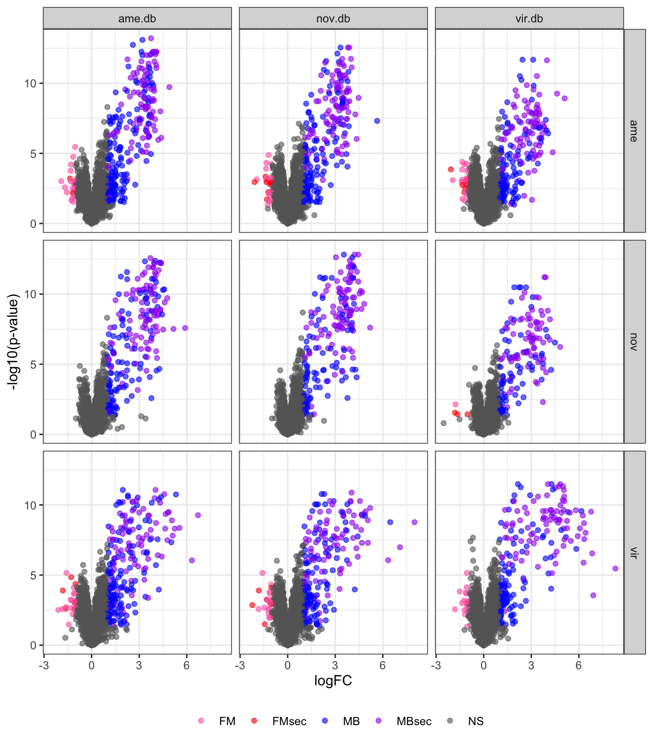
| Version | Author | Date |
|---|---|---|
| f28e7a0 | MartinGarlovsky | 2022-02-07 |
Overlap in ‘Sfps’ between species
We compare the number of ejaculate candidates detected using each species database.
ame db
# upset(fromList(list(ame = ame_DATABLES$genes[ame_DATABLES$species == 'ame' & ame_DATABLES$logFC > 1 & ame_DATABLES$adj.P.Val < 0.05],
#                     nov = ame_DATABLES$genes[ame_DATABLES$species == 'nov' & ame_DATABLES$logFC > 1 & ame_DATABLES$adj.P.Val < 0.05],
#                     vir = ame_DATABLES$genes[ame_DATABLES$species == 'vir' & ame_DATABLES$logFC > 1 & ame_DATABLES$adj.P.Val < 0.05])))

fit_ame <- euler(c('ame' = 49, "nov" = 18, "vir" = 58,
                   'ame&nov' = 51, 'ame&vir' = 29, 'nov&vir' = 1,
                   'ame&nov&vir' = 140))

#pdf('plots/sfp_overlap.pdf', height = 4, width = 4)
plot(fit_ame,
     quantities = TRUE,
     fills = list(fill = viridis::viridis(n = 3), alpha = .5))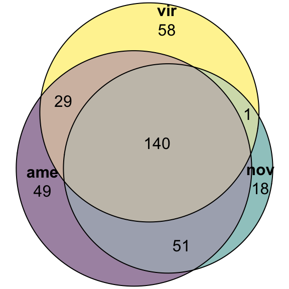
#dev.off()nov db
# upset(fromList(list(ame = nov_DATABLES$genes[nov_DATABLES$species == 'ame' & nov_DATABLES$logFC > 1 & nov_DATABLES$adj.P.Val < 0.05],
#                     nov = nov_DATABLES$genes[nov_DATABLES$species == 'nov' & nov_DATABLES$logFC > 1 & nov_DATABLES$adj.P.Val < 0.05],
#                     vir = nov_DATABLES$genes[nov_DATABLES$species == 'vir' & nov_DATABLES$logFC > 1 & nov_DATABLES$adj.P.Val < 0.05])))

fit_nov <- euler(c('ame' = 45, "nov" = 17, "vir" = 56,
                   'ame&nov' = 51, 'ame&vir' = 27, 'nov&vir' = 4,
                   'ame&nov&vir' = 122))

#pdf('plots/sfp_overlap.pdf', height = 4, width = 4)
plot(fit_nov,
     quantities = TRUE,
     fills = list(fill = viridis::viridis(n = 3), alpha = .5))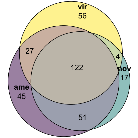
#dev.off()vir db
# upset(fromList(list(ame = vir_DATABLES$genes[vir_DATABLES$species == 'ame' & vir_DATABLES$logFC > 1 & vir_DATABLES$adj.P.Val < 0.05],
#                     nov = vir_DATABLES$genes[vir_DATABLES$species == 'nov' & vir_DATABLES$logFC > 1 & vir_DATABLES$adj.P.Val < 0.05],
#                     vir = vir_DATABLES$genes[vir_DATABLES$species == 'vir' & vir_DATABLES$logFC > 1 & vir_DATABLES$adj.P.Val < 0.05])))

fit_vir <- euler(c('ame' = 37, "nov" = 13, "vir" = 42,
                   'ame&nov' = 24, 'ame&vir' = 36, 'nov&vir' = 3,
                   'ame&nov&vir' = 109))

#pdf('plots/sfp_overlap.pdf', height = 4, width = 4)
plot(fit_vir,
     quantities = TRUE,
     fills = list(fill = viridis::viridis(n = 3), alpha = .5))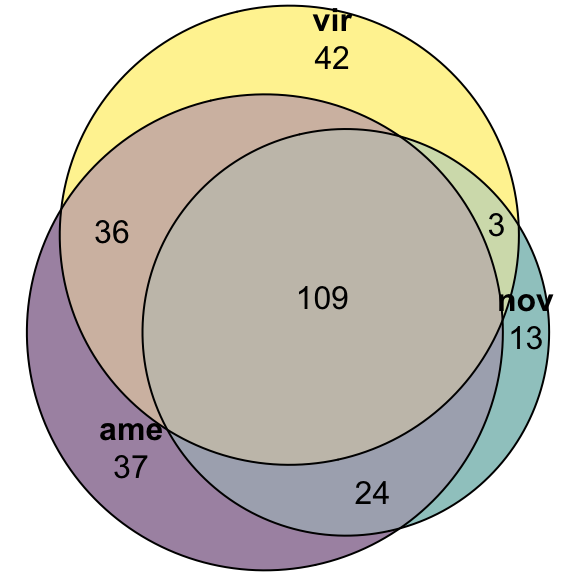
#dev.off()Plot species specific database
facet_names <- c(ame = "D. americana",
                 nov = 'D. novamexicana',
                 vir = "D. virilis")

lab_text <- data.frame(species = c('ame', 'nov', 'vir'),
                       P.Value = 1,
                       logFC = 8.8,
                       lab = c("D. americana", 'D. novamexicana', "D. virilis"),
                       DA = NA,
                       threshold = NA)

# plot
bind_rows(ame_DATABLES %>% filter(species == 'ame'),
          nov_DATABLES %>% filter(species == 'nov'),
          vir_DATABLES %>% filter(species == 'vir')) %>%
  ggplot(aes(x = logFC, y = -log10(P.Value), colour = DA, shape = threshold)) +
  geom_point(alpha = .6) +
  scale_shape_manual(values = c(16, 1), guide = 'none') +
  scale_colour_manual(values = c(viridis::plasma(n = 4, direction = -1), 'grey80')) +
  labs(y = '-log10(p-value)') +
  facet_wrap(~species, nrow = 1, labeller = as_labeller(facet_names)) +
  theme_bw() +
  theme(legend.position = '',#c(0.04, 0.8),
        legend.title = element_blank(),
        legend.background = element_rect(fill = NA),
        strip.text = element_text(size = 15, face = "italic"),
        strip.background = element_blank(),
        strip.text.x = element_blank()) +
  geom_text(data = lab_text, colour = 'black', hjust = 1,
            aes(y = -log10(P.Value), label = paste0(lab)), size = 4, fontface = "italic") +
  #ggsave('plots/volcano_mated-virgin.pdf', height = 7, width = 18, units = 'cm', dpi = 600, useDingbats = FALSE) +
  NULL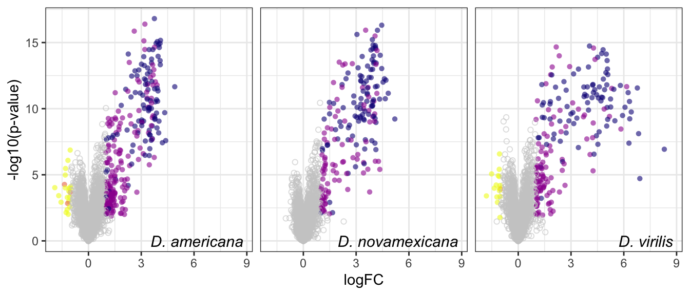
# combine ejaculate candidates with orthologs
ejac_cands <- bind_rows(ame_DATABLES %>% filter(str_detect(DA, pattern = 'MB')),
                        nov_DATABLES %>% filter(str_detect(DA, pattern = 'MB')),
                        vir_DATABLES %>% filter(str_detect(DA, pattern = 'MB'))) %>%
  drop_na(Orthogroup)

# # overlap for ejaculate candidates with orthologs using each database
# upset(fromList(list(ame.db = split(ejac_cands, ejac_cands$DB)[[1]][[13]],
#                     nov.db = split(ejac_cands, ejac_cands$DB)[[2]][[13]],
#                     vir.db = split(ejac_cands, ejac_cands$DB)[[3]][[13]])))

#pdf('plots/sfp_overlap_all_db.pdf', height = 4, width = 4)
plot(venn(c('D. ame' = 17, 'D. nov' = 6, 'D. vir' = 9,
            'D. ame&D. nov' = 18, 'D. ame&D. vir' = 4, 'D. nov&D. vir' = 5,
            'D. ame&D. nov&D. vir' = 169)
          ),
     quantities = TRUE,
     fills = list(fill = viridis::viridis(n = 3), alpha = .5))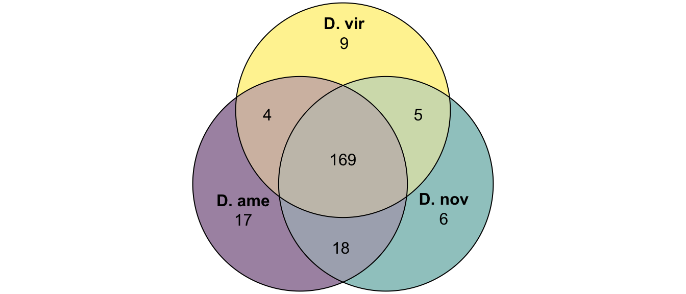
| Version | Author | Date |
|---|---|---|
| f28e7a0 | MartinGarlovsky | 2022-02-07 |
#dev.off()

# overlap in ejaculate candidates between species
bind_rows(ame_DATABLES %>% filter(str_detect(DA, pattern = 'MB')),
          nov_DATABLES %>% filter(str_detect(DA, pattern = 'MB')),
          vir_DATABLES %>% filter(str_detect(DA, pattern = 'MB'))) %>%
  mutate(orth = if_else(is.na(Orthogroup) == TRUE, 'no', 'yes')) %>%
  group_by(DB, orth) %>%
  summarise(N = n_distinct(genes)) %>%
  pivot_wider(id_cols = DB, names_from = orth, values_from = N) %>%
  mutate(prop.orths = yes/(yes + no),
         no.orths = 1 - prop.orths) %>%
  kable(digits = 3,
        caption = 'Numbers and proportions of ejaculate candidates in each species with or without orthologs') %>%
kable_styling(full_width = FALSE)| DB | no | yes | prop.orths | no.orths |
|---|---|---|---|---|
| ame.db | 138 | 208 | 0.601 | 0.399 |
| nov.db | 124 | 198 | 0.615 | 0.385 |
| vir.db | 77 | 187 | 0.708 | 0.292 |
#number of ejaculate candidates using each species database including without orthologs
ejac_ids <- bind_rows(ame_DATABLES %>% filter(str_detect(DA, pattern = 'MB')),
                      nov_DATABLES %>% filter(str_detect(DA, pattern = 'MB')),
                      vir_DATABLES %>% filter(str_detect(DA, pattern = 'MB'))) %>%
  mutate(OrthID = if_else(is.na(Orthogroup) == TRUE, paste0(genes, species), Orthogroup)) %>%
  distinct(genes, DB, .keep_all = TRUE) %>% drop_na(Orthogroup)

# total number of unique ejaculate candidates identified
#n_distinct(ejac_ids$OrthID)

# upset(fromList(list(ame = split(ejac_ids, ejac_ids$DB)[[1]][[15]],
#                     nov = split(ejac_ids, ejac_ids$DB)[[2]][[15]],
#                     vir = split(ejac_ids, ejac_ids$DB)[[3]][[15]])))

#pdf('plots/sfp_overlap_all_db_noOrths.pdf', height = 4, width = 4)
plot(venn(c('D. ame' = 155, 'D. nov' = 130, 'D. vir' = 86,
            'D. ame&D. nov' = 18, 'D. ame&D. vir' = 4, 'D. nov&D. vir' = 5,
            'D. ame&D. nov&D. vir' = 169)
          ),
     quantities = TRUE,
     fills = list(fill = viridis::viridis(n = 3), alpha = .5))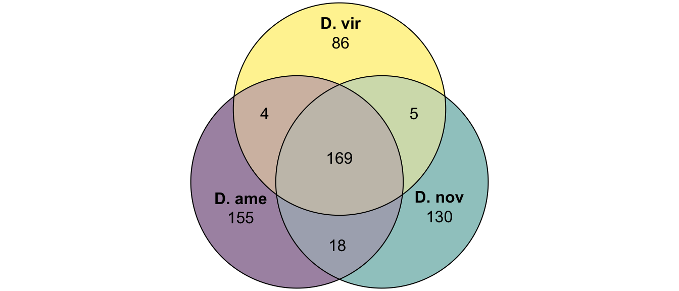
| Version | Author | Date |
|---|---|---|
| f28e7a0 | MartinGarlovsky | 2022-02-07 |
#dev.off()

# number and proportion secreted
bind_rows(ame_DATABLES %>% filter(str_detect(DA, pattern = 'MB')),
          nov_DATABLES %>% filter(str_detect(DA, pattern = 'MB')),
          vir_DATABLES %>% filter(str_detect(DA, pattern = 'MB'))) %>%
  distinct(genes, DB, .keep_all = TRUE) %>%
  group_by(DB, DA) %>% dplyr::count() %>%
  pivot_wider(id_cols = DB, names_from = DA, values_from = n) %>%
  mutate(prop.sec = MBsec/(MBsec + MB)) %>%
  kable(digits = 3,
        caption = 'The number of proteins higher in abundance in mated comapred to virgin samples with or without a secretion signal using each species database') %>%
kable_styling(full_width = FALSE)| DB | MB | MBsec | prop.sec |
|---|---|---|---|
| ame.db | 233 | 113 | 0.327 |
| nov.db | 198 | 124 | 0.385 |
| vir.db | 160 | 104 | 0.394 |
# #write FBgns for ClueGO - ejaculate candidates
# ejac_cands %>% distinct(FBgn, .keep_all = TRUE) %>%
#   write_csv('output/ClueGOlists/all_ejac_FBgn.csv')

# # proteins higher abundance in FRT
# bind_rows(ame_DATABLES %>% filter(str_detect(DA, pattern = 'FM')),
#           nov_DATABLES %>% filter(str_detect(DA, pattern = 'FM')),
#           vir_DATABLES %>% filter(str_detect(DA, pattern = 'FM'))) %>%
#   drop_na(Orthogroup) %>%
#   distinct(FBgn, .keep_all = TRUE) %>%
#   write_csv('output/ClueGOlists/virgin_biased_FBgn.csv')
Sfp overlap with previous studies
We compare the number of putative seminal fluid proteins identified in previous studies in the virilis group from Ahmed-Braimah et al. 2017 and Ahmed-Braimah et al. 2021.
overlap with Ahmed-Braimah et al. 2017
# upset(fromList(list(proteomic = c(vir_DATABLES %>%
#                                     filter(str_detect(DA, pattern = 'MB')) %>% distinct(FBgn))$FBgn,
#                     AG_biased = Dvir_SFPs$FBgn[Dvir_SFPs$bias == 'AG-biased'],
#                     EB_biased = Dvir_SFPs$FBgn[Dvir_SFPs$bias == 'EB-biased'],
#                     SFP       = Dvir_SFPs$FBgn[Dvir_SFPs$bias == 'SFP'])))

#pdf('plots/sfp_orth_overlap.pdf', height = 4, width = 4)
plot(euler(c('AG' = 102, "EB" = 86, "Prot" = 130, 'SFP' = 42,
                'SFP&Prot' = 29, 'AG&Prot' = 17, 'EB&Prot' = 6)
              ),
     quantities = TRUE,
     fills = list(fill = c("turquoise", "orange", "red", 'purple'), alpha = .5))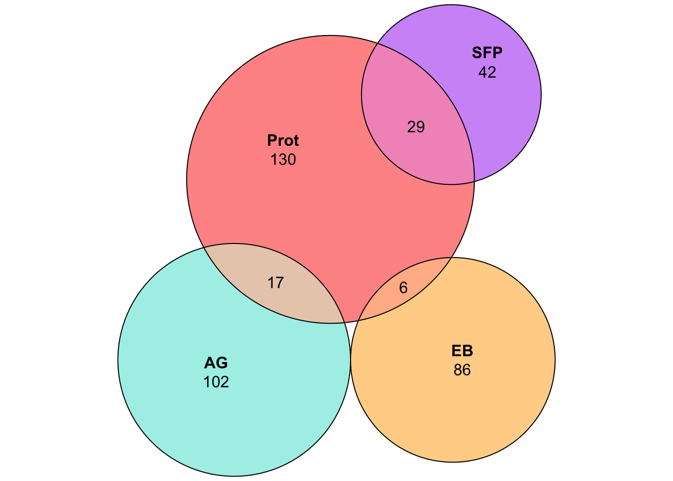
#dev.off()Overlap with female reproductive tract genes
# upset(fromList(list(proteomic = c(bind_rows(ame_DATABLES, nov_DATABLES, vir_DATABLES) %>% pull(FBgn)),
#                     FRT_biased = FRTbiased$FBgn_ID,
#                     PMR_biased = virilisPMDE$FBgn_ID)))

plot(euler(c('FRT' = 82, "PMR" = 323, "PRO" = 2356,
             'FRT&PMR' = 14, 'FRT&PRO' = 50, 'PRO&PMR' = 104,
             'FRT&PMR&PRO' = 2)
              ),
     quantities = TRUE,
     fills = list(fill = c("orange", "red", 'purple'), alpha = .5))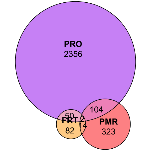
Divergence between ejaculate candidates
We performed differential abundance analysis between species for mated samples to identify differences in the male ejaculate between species. We subset the data to include only ‘ejaculate candidates’ - i.e. proteins significantly higher abundance in mated compared to virgin samples. We performed analyses using each species database and using the ‘combined database’.
# subset data to only include ejaculate candidates
ame_mated <- ame_abund %>% dplyr::select(Accession, unique.p, contains('M')) %>%
  filter(Accession %in% ejac_cands$genes[ejac_cands$DB == 'ame.db'])

nov_mated <- nov_abund %>% dplyr::select(Accession, unique.p, contains('M')) %>%
  filter(Accession %in% ejac_cands$genes[ejac_cands$DB == 'nov.db'])

vir_mated <- vir_abund %>% dplyr::select(Accession, unique.p, contains('M')) %>%
  filter(Accession %in% ejac_cands$genes[ejac_cands$DB == 'vir.db'])

# get sample info - same for all db's
sampInfo.m <- data.frame(condition = str_sub(colnames(ame_mated[3:11]), 1, 2),
                         Replicate = str_sub(colnames(ame_mated[3:11]), 3, 3))

# make design matrix to test diffs between groups
design.m <- model.matrix(~0 + sampInfo.m$condition)
colnames(design.m) <- unique(sampInfo.m$condition)
rownames(design.m) <- sampInfo.m$Replicate

# make contrasts - higher values = higher in mated
cont.mated <- makeContrasts(a.m.n = AM - NM,
                            a.m.v = AM - VM,
                            n.m.v = NM - VM,
                            levels = design.m)

# create DGElist and fit model
dge_ame.m <- DGEList(counts = ame_mated[, 3:11], genes = ame_mated$Accession, group = sampInfo.m$condition)
dge_nov.m <- DGEList(counts = nov_mated[, 3:11], genes = nov_mated$Accession, group = sampInfo.m$condition)
dge_vir.m <- DGEList(counts = vir_mated[, 3:11], genes = vir_mated$Accession, group = sampInfo.m$condition)

dge_ame.m <- calcNormFactors(dge_ame.m, method = 'TMM')
dge_nov.m <- calcNormFactors(dge_nov.m, method = 'TMM')
dge_vir.m <- calcNormFactors(dge_vir.m, method = 'TMM')

dge_ame.m <- estimateCommonDisp(dge_ame.m)
dge_nov.m <- estimateCommonDisp(dge_nov.m)
dge_vir.m <- estimateCommonDisp(dge_vir.m)

dge_ame.m <- estimateTagwiseDisp(dge_ame.m)
dge_nov.m <- estimateTagwiseDisp(dge_nov.m)
dge_vir.m <- estimateTagwiseDisp(dge_vir.m)

# voom normalisation
dge_ame.m <- voom(dge_ame.m, design.m, plot = FALSE)
dge_nov.m <- voom(dge_nov.m, design.m, plot = FALSE)
dge_vir.m <- voom(dge_vir.m, design.m, plot = FALSE)

# fit linear model
lm_ame.m <- lmFit(dge_ame.m, design = design.m)
lm_nov.m <- lmFit(dge_nov.m, design = design.m)
lm_vir.m <- lmFit(dge_vir.m, design = design.m)

# compare DA between mated samples

# ame using each database
mated_an2ame <- contrasts.fit(lm_ame.m, cont.mated[,"a.m.n"])
mated_an2nov <- contrasts.fit(lm_nov.m, cont.mated[,"a.m.n"])
mated_an2vir <- contrasts.fit(lm_vir.m, cont.mated[,"a.m.n"])

mated_an2ame <- eBayes(mated_an2ame)
mated_an2nov <- eBayes(mated_an2nov)
mated_an2vir <- eBayes(mated_an2vir)

mated_an2ame.tTags.table <- topTable(mated_an2ame, adjust.method = "BH", number = Inf)
mated_an2nov.tTags.table <- topTable(mated_an2nov, adjust.method = "BH", number = Inf)
mated_an2vir.tTags.table <- topTable(mated_an2vir, adjust.method = "BH", number = Inf)

# nov using each database
mated_av2ame <- contrasts.fit(lm_ame.m, cont.mated[,"a.m.v"])
mated_av2nov <- contrasts.fit(lm_nov.m, cont.mated[,"a.m.v"])
mated_av2vir <- contrasts.fit(lm_vir.m, cont.mated[,"a.m.v"])

mated_av2ame <- eBayes(mated_av2ame)
mated_av2nov <- eBayes(mated_av2nov)
mated_av2vir <- eBayes(mated_av2vir)

mated_av2ame.tTags.table <- topTable(mated_av2ame, adjust.method = "BH", number = Inf)
mated_av2nov.tTags.table <- topTable(mated_av2nov, adjust.method = "BH", number = Inf)
mated_av2vir.tTags.table <- topTable(mated_av2vir, adjust.method = "BH", number = Inf)

# vir using each database
mated_nv2ame <- contrasts.fit(lm_ame.m, cont.mated[,"n.m.v"])
mated_nv2nov <- contrasts.fit(lm_nov.m, cont.mated[,"n.m.v"])
mated_nv2vir <- contrasts.fit(lm_vir.m, cont.mated[,"n.m.v"])

mated_nv2ame <- eBayes(mated_nv2ame)
mated_nv2nov <- eBayes(mated_nv2nov)
mated_nv2vir <- eBayes(mated_nv2vir)

mated_nv2ame.tTags.table <- topTable(mated_nv2ame, adjust.method = "BH", number = Inf)
mated_nv2nov.tTags.table <- topTable(mated_nv2nov, adjust.method = "BH", number = Inf)
mated_nv2vir.tTags.table <- topTable(mated_nv2vir, adjust.method = "BH", number = Inf)

# combine results
ame_MATED <- rbind(mated_an2ame.tTags.table %>% mutate(comparison = 'ame.v.nov'),
                   mated_av2ame.tTags.table %>% mutate(comparison = 'ame.v.vir'),
                   mated_nv2ame.tTags.table %>% mutate(comparison = 'nov.v.vir')) %>%
  mutate(DB = 'ame.db',
         threshold = if_else(adj.P.Val < 0.05 & abs(logFC) > 1, 'DA', 'NS'),
         # add variable for signal peptides
         sigP = if_else(genes %in% signal_peps_ame$ID, 'sigP', 'not'),
         DA = case_when(sigP == 'sigP' & threshold == 'DA' ~ 'sigP',
                        threshold == 'DA' ~ 'DA',
                        TRUE ~ 'NS'))

nov_MATED <- rbind(mated_an2nov.tTags.table %>% mutate(comparison = 'ame.v.nov'),
                   mated_av2nov.tTags.table %>% mutate(comparison = 'ame.v.vir'),
                   mated_nv2nov.tTags.table %>% mutate(comparison = 'nov.v.vir')) %>%
  mutate(DB = 'nov.db',
         threshold = if_else(adj.P.Val < 0.05 & abs(logFC) > 1, 'DA', 'NS'),
         # add variable for signal peptides
         sigP = if_else(genes %in% signal_peps_nov$ID, 'sigP', 'not'),
         DA = case_when(sigP == 'sigP' & threshold == 'DA' ~ 'sigP',
                        threshold == 'DA' ~ 'DA',
                        TRUE ~ 'NS'))

vir_MATED <- rbind(mated_an2vir.tTags.table %>% mutate(comparison = 'ame.v.nov'),
                   mated_av2vir.tTags.table %>% mutate(comparison = 'ame.v.vir'),
                   mated_nv2vir.tTags.table %>% mutate(comparison = 'nov.v.vir')) %>%
  mutate(DB = 'vir.db',
         threshold = if_else(adj.P.Val < 0.05 & abs(logFC) > 1, 'DA', 'NS'),
         # add variable for signal peptides
         sigP = if_else(genes %in% signal_peps_vir$ID, 'sigP', 'not'),
         DA = case_when(sigP == 'sigP' & threshold == 'DA' ~ 'sigP',
                        threshold == 'DA' ~ 'DA',
                        TRUE ~ 'NS'))
Volcano plots all vs. all
Compare results using each species database
bind_rows(ame_MATED,
          nov_MATED,
          vir_MATED) %>%
  ggplot(aes(x = logFC, y = -log10(adj.P.Val), colour = DA)) +
  geom_point(alpha = .6) +
  scale_colour_manual(values = c('hotpink', 'grey40', 'red')) +
  labs(y = '-log10(p-value)') +
  facet_grid(comparison ~ DB) +
  theme_bw() +
  theme(#legend.position = '',
        legend.title = element_blank(),
        legend.background = element_rect(fill = NA)) +
  NULL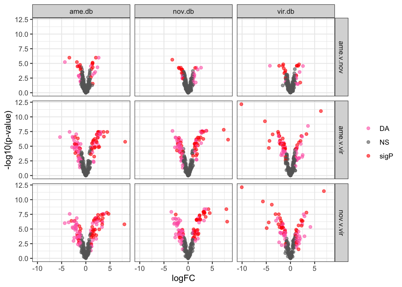
number of DA in one species vs. other
bind_rows(ame_MATED,
          nov_MATED,
          vir_MATED) %>% filter(threshold != 'NS') %>%
  mutate(up = ifelse(logFC > 1, 'a', 'b')) %>%
  group_by(comparison, DB, up) %>% dplyr::count() %>%
  ggplot(aes(x = up, y = n, fill = up)) +
  geom_col() +
  facet_grid(comparison ~ DB)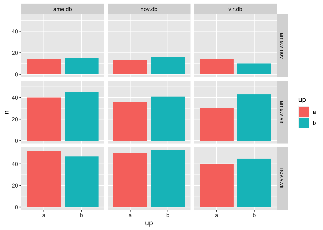
We tested whether signal peptides are more likely to be differentially abundant between species than other proteins
bind_rows(ame_MATED,
          nov_MATED,
          vir_MATED) %>%
  group_by(comparison, DB, threshold, sigP) %>% dplyr::count() %>%
  ggplot(aes(x = sigP, y = n, fill = threshold)) +
  geom_col(position = 'fill') +
  facet_grid(comparison ~ DB)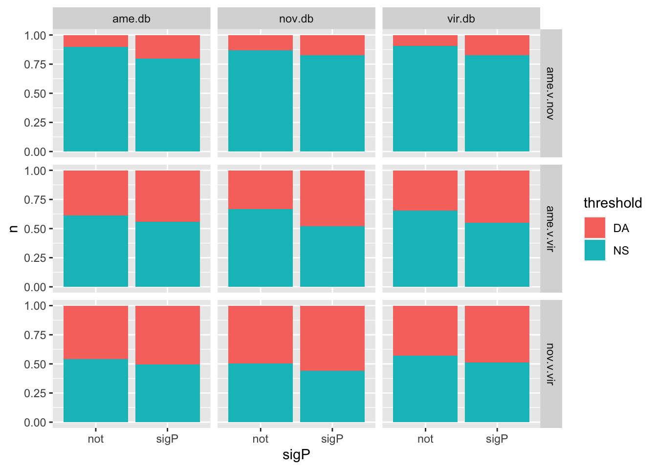
# do Fisher's exact tests
fish_sig <- bind_rows(
  ame_MATED %>%
    group_by(comparison) %>%
    do(fit = broom::tidy(fisher.test(as.matrix(xtabs(~ threshold + sigP, ., sparse = T))))) %>%
    unnest(fit) %>%
    mutate(db = 'ame.db'),
  nov_MATED %>%
    group_by(comparison) %>%
    do(fit = broom::tidy(fisher.test(as.matrix(xtabs(~ threshold + sigP, ., sparse = T))))) %>%
    unnest(fit) %>%
    mutate(db = 'nov.db'),
  ame_MATED %>%
    group_by(comparison) %>%
    do(fit = broom::tidy(fisher.test(as.matrix(xtabs(~ threshold + sigP, ., sparse = T))))) %>%
    unnest(fit) %>%
         mutate(db = 'vir.db'))

fish_sig$FDR <- p.adjust(fish_sig$p.value, method = 'fdr')

fish_sig %>%
  mutate(p.val = ifelse(FDR < 0.001, '< 0.001', round(FDR, 3)),
         comparison = recode(comparison,
                      ame.v.nov = "D. ame vs. D. nov",
                      ame.v.vir = "D. ame vs. D. vir",
                      nov.v.vir = 'D. nov vs. D. vir'),
         across(2:5, ~ round(.x, 2)),
         Estimate = paste0(estimate, ' (', conf.low, '-', conf.high, ')')) %>%
  dplyr::select(comparison, Estimate, p.val) %>%
  kable(digits = 3,
        caption = 'Fisher\'s exact tests corrected for multiple testing') %>%
kable_styling(full_width = FALSE)| comparison | Estimate | p.val |
|---|---|---|
| D. ame vs. D. nov | 0.44 (0.18-1.05) | 0.185 |
| D. ame vs. D. vir | 0.8 (0.43-1.46) | 0.568 |
| D. nov vs. D. vir | 0.82 (0.45-1.5) | 0.568 |
| D. ame vs. D. nov | 0.71 (0.3-1.73) | 0.568 |
| D. ame vs. D. vir | 0.54 (0.29-1.02) | 0.185 |
| D. nov vs. D. vir | 0.77 (0.42-1.43) | 0.568 |
| D. ame vs. D. nov | 0.44 (0.18-1.05) | 0.185 |
| D. ame vs. D. vir | 0.8 (0.43-1.46) | 0.568 |
| D. nov vs. D. vir | 0.82 (0.45-1.5) | 0.568 |
Divergence between (virgin) female reproductive tracts
Here we compare abundance of proteins in virgin samples after filtering out “ejaculate candidates”.
# already filtered 2 unique peptides
ame_virgin <- ame_abund %>% filter(!Accession %in% ejac_cands$genes[ejac_cands$DB == 'ame.db']) %>%
  dplyr::select(Accession, unique.p, !contains('M'))
nov_virgin <- nov_abund %>% filter(!Accession %in% ejac_cands$genes[ejac_cands$DB == 'nov.db']) %>%
  dplyr::select(Accession, unique.p, !contains('M'))
vir_virgin <- vir_abund %>% filter(!Accession %in% ejac_cands$genes[ejac_cands$DB == 'vir.db']) %>%
  dplyr::select(Accession, unique.p, !contains('M'))

# get sample info - same for all db's
sampInfo.v = data.frame(condition = str_sub(colnames(ame_virgin[-c(1:2)]), 1, 2),
                        Replicate = str_sub(colnames(ame_virgin[-c(1:2)]), 3, 3))

# make design matrix to test diffs between groups
design.v <- model.matrix(~0 + sampInfo.v$condition)
colnames(design.v) <- unique(sampInfo.v$condition)
rownames(design.v) <- sampInfo.v$Replicate

# make contrasts - higher values = higher in mated
cont.virgin <- makeContrasts(a.v.n = AV - NV,
                             a.v.v = AV - VV,
                             n.v.v = NV - VV,
                             levels = design.v)

# create DGElist and fit model
dge_ame.v <- DGEList(counts = ame_virgin[, -c(1:2)], genes = ame_virgin$Accession, group = sampInfo.v$condition)
dge_nov.v <- DGEList(counts = nov_virgin[, -c(1:2)], genes = nov_virgin$Accession, group = sampInfo.v$condition)
dge_vir.v <- DGEList(counts = vir_virgin[, -c(1:2)], genes = vir_virgin$Accession, group = sampInfo.v$condition)

dge_ame.v <- calcNormFactors(dge_ame.v, method = 'TMM')
dge_nov.v <- calcNormFactors(dge_nov.v, method = 'TMM')
dge_vir.v <- calcNormFactors(dge_vir.v, method = 'TMM')

dge_ame.v <- estimateCommonDisp(dge_ame.v)
dge_nov.v <- estimateCommonDisp(dge_nov.v)
dge_vir.v <- estimateCommonDisp(dge_vir.v)

dge_ame.v <- estimateTagwiseDisp(dge_ame.v)
dge_nov.v <- estimateTagwiseDisp(dge_nov.v)
dge_vir.v <- estimateTagwiseDisp(dge_vir.v)

# voom normalisation
dge_ame.v <- voom(dge_ame.v, design.v, plot = FALSE)
dge_nov.v <- voom(dge_nov.v, design.v, plot = FALSE)
dge_vir.v <- voom(dge_vir.v, design.v, plot = FALSE)

# fit linear model
lm_ame.v <- lmFit(dge_ame.v, design = design.v)
lm_nov.v <- lmFit(dge_nov.v, design = design.v)
lm_vir.v <- lmFit(dge_vir.v, design = design.v)

# compare DA between virgin samples

# ame using each database
virgin_an2ame <- contrasts.fit(lm_ame.v, cont.virgin[,"a.v.n"])
virgin_an2nov <- contrasts.fit(lm_nov.v, cont.virgin[,"a.v.n"])
virgin_an2vir <- contrasts.fit(lm_vir.v, cont.virgin[,"a.v.n"])

virgin_an2ame <- eBayes(virgin_an2ame)
virgin_an2nov <- eBayes(virgin_an2nov)
virgin_an2vir <- eBayes(virgin_an2vir)

virgin_an2ame.tTags.table <- topTable(virgin_an2ame, adjust.method = "BH", number = Inf)
virgin_an2nov.tTags.table <- topTable(virgin_an2nov, adjust.method = "BH", number = Inf)
virgin_an2vir.tTags.table <- topTable(virgin_an2vir, adjust.method = "BH", number = Inf)

# nov using each database
virgin_av2ame <- contrasts.fit(lm_ame.v, cont.virgin[,"a.v.v"])
virgin_av2nov <- contrasts.fit(lm_nov.v, cont.virgin[,"a.v.v"])
virgin_av2vir <- contrasts.fit(lm_vir.v, cont.virgin[,"a.v.v"])

virgin_av2ame <- eBayes(virgin_av2ame)
virgin_av2nov <- eBayes(virgin_av2nov)
virgin_av2vir <- eBayes(virgin_av2vir)

virgin_av2ame.tTags.table <- topTable(virgin_av2ame, adjust.method = "BH", number = Inf)
virgin_av2nov.tTags.table <- topTable(virgin_av2nov, adjust.method = "BH", number = Inf)
virgin_av2vir.tTags.table <- topTable(virgin_av2vir, adjust.method = "BH", number = Inf)

# vir using each database
virgin_nv2ame <- contrasts.fit(lm_ame.v, cont.virgin[,"n.v.v"])
virgin_nv2nov <- contrasts.fit(lm_nov.v, cont.virgin[,"n.v.v"])
virgin_nv2vir <- contrasts.fit(lm_vir.v, cont.virgin[,"n.v.v"])

virgin_nv2ame <- eBayes(virgin_nv2ame)
virgin_nv2nov <- eBayes(virgin_nv2nov)
virgin_nv2vir <- eBayes(virgin_nv2vir)

virgin_nv2ame.tTags.table <- topTable(virgin_nv2ame, adjust.method = "BH", number = Inf)
virgin_nv2nov.tTags.table <- topTable(virgin_nv2nov, adjust.method = "BH", number = Inf)
virgin_nv2vir.tTags.table <- topTable(virgin_nv2vir, adjust.method = "BH", number = Inf)

# combine results
ame_VIRGIN <- rbind(virgin_an2ame.tTags.table %>% mutate(comparison = 'ame.v.nov'),
                    virgin_av2ame.tTags.table %>% mutate(comparison = 'ame.v.vir'),
                    virgin_nv2ame.tTags.table %>% mutate(comparison = 'nov.v.vir')) %>%
  mutate(DB = 'ame.db',
         threshold = if_else(adj.P.Val < 0.05 & abs(logFC) > 1, 'DA', 'NS'),
         # add variable for signal peptides reaching significance threshold
         sigP = case_when(genes %in% signal_peps_ame$ID & threshold == 'DA' ~ 'sigP',
                          threshold == 'DA' ~ 'DA',
                          TRUE ~ 'NS'))

nov_VIRGIN <- rbind(virgin_an2nov.tTags.table %>% mutate(comparison = 'ame.v.nov'),
                    virgin_av2nov.tTags.table %>% mutate(comparison = 'ame.v.vir'),
                    virgin_nv2nov.tTags.table %>% mutate(comparison = 'nov.v.vir')) %>%
  mutate(DB = 'nov.db',
         threshold = if_else(adj.P.Val < 0.05 & abs(logFC) > 1, 'DA', 'NS'),
         # add variable for signal peptides reaching significance threshold
         sigP = case_when(genes %in% signal_peps_nov$ID & threshold == 'DA' ~ 'sigP',
                          threshold == 'DA' ~ 'DA',
                          TRUE ~ 'NS'))

vir_VIRGIN <- rbind(virgin_an2vir.tTags.table %>% mutate(comparison = 'ame.v.nov'),
                    virgin_av2vir.tTags.table %>% mutate(comparison = 'ame.v.vir'),
                    virgin_nv2vir.tTags.table %>% mutate(comparison = 'nov.v.vir')) %>%
  mutate(DB = 'vir.db',
         threshold = if_else(adj.P.Val < 0.05 & abs(logFC) > 1, 'DA', 'NS'),
         # add variable for signal peptides reaching significance threshold
    sigP = case_when(genes %in% signal_peps_vir$ID & threshold == 'DA' ~ 'sigP',
                     threshold == 'DA' ~ 'DA',
                     TRUE ~ 'NS'))

# plot all vs. all
bind_rows(ame_VIRGIN,
          nov_VIRGIN,
          vir_VIRGIN) %>%
  ggplot(aes(x = logFC, y = -log10(adj.P.Val), colour = sigP)) +
  geom_point(alpha = .6) +
  scale_colour_manual(values = c('hotpink', 'grey40', 'red')) +
  labs(y = '-log10(p-value)') +
  facet_grid(comparison ~ DB) +
  theme_bw() +
  theme(#legend.position = '',
        legend.title = element_blank(),
        legend.background = element_rect(fill = NA)) +
  NULL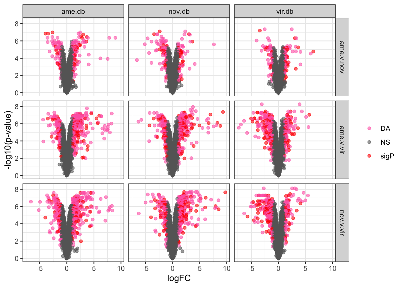
Multi-database analysis
Here we perform differential abundance analyses using the combined database using species-specific abundance data collated using each iterative run from Proteome Discoverer. We filter to only include proteins identified by two or more unique peptides.
multiDB <- recip_dat %>%
  dplyr::select(FBgn, Accession_vir, Orthogroup, starts_with('Number.of.Unique.Peptides'),
                AM1_ame, AM2_ame, AM3_ame, AV1_ame, AV2_ame,
                NM1_nov, NM2_nov, NM3_nov, NV1_nov, NV2_nov,
                VM1_vir, VM2_vir, VM3_vir, VV1_vir, VV2_vir, VV3_vir)

colnames(multiDB) <- gsub('Number.of.Unique.Peptides', 'UP', x = colnames(multiDB))
colnames(multiDB)[7:22] <- gsub('_.*', '', x = colnames(multiDB)[7:22])

# filter must have two unique peptides in at least 1 dataset
multiDB2 <- multiDB %>%
  filter(UP_ame >= 2 | UP_nov >= 2 | UP_vir >= 2) %>%
  mutate(across(7:22, ~replace_na(.x, 0)))

# make object for protein abundance data and replace NA's with 0's
expr_data <- multiDB2[, -c(1:6)]

# get sample info
sampInfo = data.frame(species = str_sub(colnames(expr_data), 1, 1),
                      mating = str_sub(colnames(expr_data), 2, 2),
                      condition = str_sub(colnames(expr_data), 1, 2),
                      Replicate = str_sub(colnames(expr_data), -1))

# make design matrix to test diffs between groups
design <- model.matrix(~0 + sampInfo$condition)
colnames(design) <- unique(sampInfo$condition)
rownames(design) <- sampInfo$Replicate

# create DGElist and fit model
dgeList <- DGEList(counts = expr_data, genes = multiDB2$Accession_vir, group = sampInfo$condition)
dgeList <- calcNormFactors(dgeList, method = 'TMM')
dgeList <- estimateCommonDisp(dgeList)
dgeList <- estimateTagwiseDisp(dgeList)

# make contrasts - higher values = higher in mated
cont.matrix <- makeContrasts(M.a.V = AM - AV,
                             M.n.V = NM - NV,
                             M.v.V = VM - VV,
                             levels = design)

# voom normalisation
dgeListV <- voom(dgeList, design, plot = FALSE)

# fit linear model
lm_fit <- lmFit(dgeListV, design = design)
Heatmap
# make DF
sample_medians <- data.frame(genes = dgeListV$genes,
                             dgeListV$E) %>%
  rowwise() %>%
  mutate(AM = median(c(!!! rlang::syms(grep('AM', names(.), value=TRUE)))),
         NM = median(c(!!! rlang::syms(grep('NM', names(.), value=TRUE)))),
         VM = median(c(!!! rlang::syms(grep('VM', names(.), value=TRUE)))),
         AV = median(c(!!! rlang::syms(grep('AV', names(.), value=TRUE)))),
         NV = median(c(!!! rlang::syms(grep('NV', names(.), value=TRUE)))),
         VV = median(c(!!! rlang::syms(grep('VV', names(.), value=TRUE))))) %>%
  dplyr::select(genes, AM, NM, VM, AV, NV, VV) %>%
  left_join(vir_ids %>% dplyr::select(prot_id, FBgn), by = c('genes' = 'prot_id')) %>%
  # add mel Sfp ortholog
  left_join(wigbySFP %>% dplyr::select(FBgn, mel_Sfp = Symbol)) %>%
  # add annotations
  mutate(Ejac = ifelse(genes %in% c(ejac_cands$genes), 'Ejac', NA),
         sperm = ifelse(genes %in% sperm_mel$prot_id, 'sperm', NA),
         sigP = ifelse(genes %in% vir_sig$ID, 'sig', NA),
         #mel_Sfp = ifelse(FBgn %in% wigbySFP$FBgn, 'Sfp', NA),
         category = case_when(genes %in% sperm_mel$prot_id ~ 'sperm',
                              FBgn %in% wigbySFP$FBgn ~ 'Sfp',
                              genes %in% vir_sig$ID ~ 'sigP',
                              TRUE ~ 'other'))

samp_hm <- sample_medians %>% dplyr::select(genes, FBgn, 2:7, mel_Sfp, category)

row.names(samp_hm) <- sample_medians$genes

mat_scaled <- t(apply(sample_medians[, 2:7], 1, scale))
colnames(mat_scaled) <- colnames(sample_medians[, 2:7])

labs1 <- rowAnnotation(cat_lab = sample_medians$category,
                       col = list(cat_lab = c(sperm = v.pal[2],
                                              Sfp = v.pal[3],
                                              sigP = v.pal[1],
                                              other = NA)),
                       Sfp_labs = anno_mark(at = c(grep('Sfp', x = sample_medians$category)),
                                            labels = sample_medians$mel_Sfp[sample_medians$category == 'Sfp'],
                                            labels_gp = gpar(fontsize = 5)),
                       title = NULL,
                       show_annotation_name = FALSE)

haha <- HeatmapAnnotation(species = str_sub(colnames(samp_hm[, 3:8]), 1, 1),
                          mating = str_sub(colnames(samp_hm[, 3:8]), 2, 2),
                          col = list(species = c('V' = v.pal[1],
                                                 'N' = v.pal[2],
                                                 'A' = v.pal[3]),
                                     mating = c('M' = viridis::magma(n = 4)[3],
                                                'V' = viridis::magma(n = 4)[2])))

#pdf('plots/all_compheatmap.pdf', height = 8, width = 5)
Heatmap(mat_scaled,
        col = viridis::inferno(100),
        heatmap_legend_param = list(title = "log2(intensities)",
                                    title_position = "leftcenter-rot"),
        right_annotation = labs1,
        top_annotation = haha,
        show_row_names = FALSE,
        show_column_names = FALSE,
        column_split = 3,
        column_gap = unit(0, "mm"),
        row_title = NULL,
        column_title = NULL)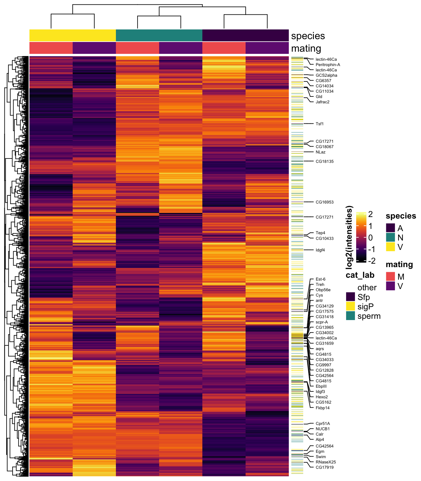
#dev.off()Diagnostic plots
par(mfrow=c(2,2))
# Biological coefficient of variation
plotBCV(dgeList)
# mean-variance trend
voomed = voom(dgeList, design, plot=TRUE)
# QQ-plot
g <- gof(glmFit(dgeList, design))
z <- zscoreGamma(g$gof.statistics,shape=g$df/2,scale=2)
qqnorm(z); qqline(z, col = 4,lwd=1,lty=1)
# log2 transformed and normalize boxplot of counts across samples
boxplot(voomed$E, xlab="", ylab="log2(Abundance)",las=2,main="Voom transformed logCPM",
        col = c(rep(brewer.pal(n = 6, name = 'Spectral'), each = 3)[-c(6,12)]))
abline(h=median(voomed$E),col="blue")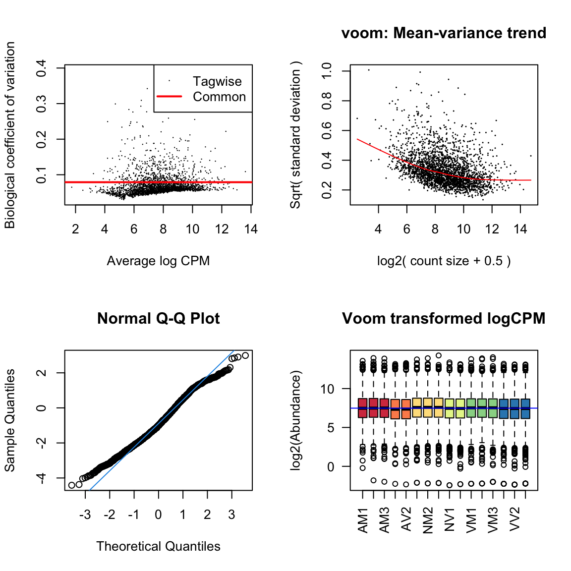
| Version | Author | Date |
|---|---|---|
| f28e7a0 | MartinGarlovsky | 2022-02-07 |
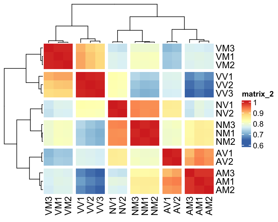
par(mfrow=c(1,1))Correlation plot
## Plot sample correlation
data = dgeListV$E %>% as_tibble()
data = as.matrix(data)
sample_cor = cor(data, method='pearson', use='pairwise.complete.obs')

pheatmap(
  mat               = sample_cor,
  border_color      = NA,
  annotation_legend = TRUE,
  annotation_names_col = FALSE,
  annotation_names_row = FALSE,
  cutree_rows = 6,
  cutree_cols = 6,
  fontsize          = 12#, file = "plots/sample.cor.pdf", height = 5.5, width = 6.5
)
Principal component analysis
pca <- prcomp(t(data), center = TRUE, scale. = TRUE)
#summary(pca)

PCA_dat <- as.data.frame(pca$x)[, 1:3] %>%
  rownames_to_column() %>%
  mutate(species = str_sub(rowname, 1, 1),
         mating = str_sub(rowname, 2, 2),
         condition = str_sub(rowname, 1, 2))

# # Plot for figure
# PCA_dat %>%
#   ggplot(aes(x = PC1, y = PC2, colour = species, shape = mating)) +
#   geom_point(size = 8, alpha = .7) +
#   labs(x = "PC1 (38.6%)", y = "PC2 (26.7%)") +
#   lims(x = c(-35, 45), y = c(-45, 45)) +
#   scale_colour_viridis_d(labels = c(expression(italic('D. ame')),
#                                     expression(italic('D. nov')),
#                                     expression(italic('D. vir')))) +
#   scale_shape_manual(values = c(16, 18), labels = c('Mated', 'Virgin')) +
#   theme_bw() +
#   theme(legend.title = element_blank(),
#         legend.text.align = 0,
#         legend.text = element_text(size = 12),
#         legend.background = element_blank(),
#         axis.text = element_text(size = 10),
#         axis.title = element_text(size = 12)) +
#   #ggsave('plots/PCA_12.pdf', height = 3.4, width = 4.8, dpi = 600, useDingbats = FALSE) +
#   NULL

rbind(as.matrix(PCA_dat[, c(2, 3)]),
      as.matrix(PCA_dat[, c(2, 4)]),
      as.matrix(PCA_dat[, c(3, 4)])) %>%
  bind_cols(species = rep(PCA_dat$species, 3),
            mating = rep(PCA_dat$mating, 3),
            pc = rep(c('PC1 (38.6%) vs. PC2 (26.7%)',
                       'PC1 (38.6%) vs. PC3 (17.9%)',
                       'PC2 (26.7%) vs. PC3 (17.9%)'), each = 16)) %>%
  ggplot(aes(x = PC1, y = PC2, colour = species, shape = mating, alpha = .5)) +
  geom_point(size = 8, alpha = .7) +
  scale_colour_viridis_d(labels = c(expression(italic('D. ame')),
                                    expression(italic('D. nov')),
                                    expression(italic('D. vir')))) +
  scale_shape_manual(values = c(16, 18), labels = c('Mated', 'Virgin')) +
  facet_wrap(~pc) +
  theme_bw() +
  theme(legend.title = element_blank(),
        legend.text.align = 0,
        legend.text = element_text(size = 12),
        legend.background = element_blank(),
        axis.text = element_text(size = 10),
        axis.title = element_blank(),
        strip.text = element_text(size = 15)) +
  #ggsave('plots/PCA_12.pdf', height = 3.4, width = 4.5, dpi = 600, useDingbats = FALSE) +
  NULL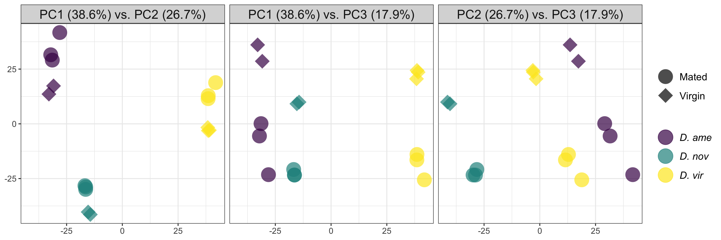
MDS plot
mdsObj <- plotMDS(dgeListV, plot = F, dim.plot = c(1,3))$cmdscale.out

mdsObj <- as.data.frame(as.matrix(mdsObj)) %>%
  rownames_to_column() %>%
  mutate(species = str_sub(rowname, 1, 1),
         mating = str_sub(rowname, 2, 2),
         condition = str_sub(rowname, 1, 2)) %>%
  dplyr::rename(dim1 = V1, dim2 = V2, dim3 = V3)

rbind(as.matrix(mdsObj[, c(2, 3)]),
      as.matrix(mdsObj[, c(2, 4)]),
      as.matrix(mdsObj[, c(3, 4)])) %>%
  bind_cols(species = rep(mdsObj$species, 3),
            mating = rep(mdsObj$mating, 3),
            dim = rep(c('Dim. 1 vs. Dim. 2',
                        'Dim. 1 vs. Dim. 3',
                        'Dim. 2 vs. Dim. 3'), each = 16)) %>%
  ggplot(aes(x = dim1, y = dim2, colour = species, shape = mating, alpha = .5)) +
  geom_point(size = 8, alpha = .7) +
  scale_colour_viridis_d(labels = c(expression(italic('D. ame')),
                                    expression(italic('D. nov')),
                                    expression(italic('D. vir')))) +
  scale_shape_manual(values = c(16, 18), labels = c('Mated', 'Virgin')) +
  facet_wrap(~dim) +
  theme_bw() +
  theme(legend.title = element_blank(),
        legend.text.align = 0,
        legend.text = element_text(size = 12),
        legend.background = element_blank(),
        axis.text = element_text(size = 10),
        axis.title = element_blank(),
        strip.text = element_text(size = 15)) +
  NULL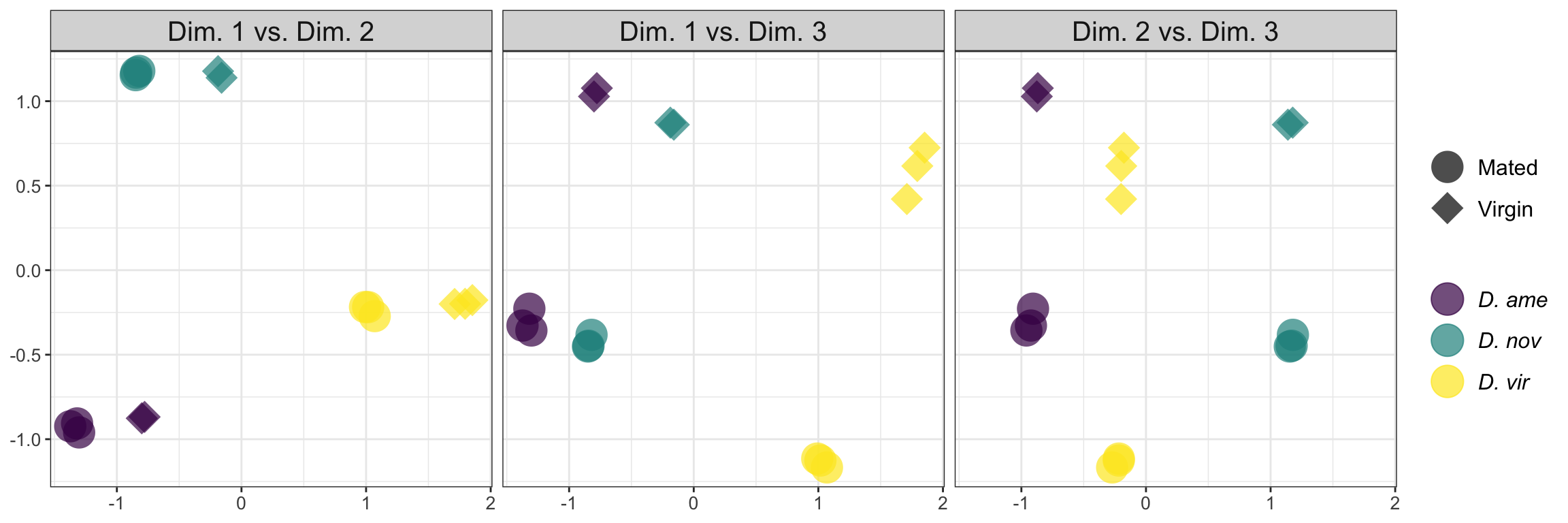
Identifying ejaculate candidates
# perform lmFit tests
# ame
lm_ame <- contrasts.fit(lm_fit, cont.matrix[,"M.a.V"])
lm_ame <- eBayes(lm_ame)
lm_ame.tTags.table <- topTable(lm_ame, adjust.method = "BH", number = Inf) %>%
  mutate(species = "ame",
         threshold = if_else(adj.P.Val < 0.05 & abs(logFC) > 1, "SD", "NS"))

# nov
lm_nov <- contrasts.fit(lm_fit, cont.matrix[,"M.n.V"])
lm_nov <- eBayes(lm_nov)
lm_nov.tTags.table <- topTable(lm_nov, adjust.method = "BH", number = Inf) %>%
  mutate(species = "nov",
         threshold = if_else(adj.P.Val < 0.05 & abs(logFC) > 1, "SD", "NS"))

# vir
lm_vir <- contrasts.fit(lm_fit, cont.matrix[,"M.v.V"])
lm_vir <- eBayes(lm_vir)
lm_vir.tTags.table <- topTable(lm_vir, adjust.method = "BH", number = Inf) %>%
  mutate(species = "vir",
         threshold = if_else(adj.P.Val < 0.05 & abs(logFC) > 1, "SD", "NS"))

comb_TABLES <- rbind(lm_ame.tTags.table,
                     lm_nov.tTags.table,
                     lm_vir.tTags.table) %>%
  left_join(multiDB2 %>% dplyr::select(FBgn, Orthogroup, Accession_vir),
            by = c('genes' = 'Accession_vir')) %>%
  mutate(
    # add variable for signal peptides reaching significance threshold
    sigP = if_else(genes %in% c(signal_peps_ame$ID,
                                signal_peps_nov$ID,
                                signal_peps_vir$ID), 'sigP', 'not'),
    # add variable splitting by bias to virgin vs. mated and signal peptide
    sperm = if_else(FBgn %in% sperm_mel$FBgn_v, 'Sperm', 'not'),
    # add variable splitting by bias to virgin vs. mated and signal peptide
    DA = case_when(threshold == 'SD' & logFC > 1 & sigP == 'sigP' ~ "MBsec",
                   threshold == 'SD' & logFC < -1 & sigP == 'sigP' ~ "FMsec",
                   threshold == 'SD' & logFC > 1 ~ "MB",
                   threshold == 'SD' & logFC < -1 ~ "FM",
                   TRUE ~ 'NS'))

## save differentially abundant proteins to table for ClueGO
# comb_TABLES %>% filter(adj.P.Val < 0.05  & logFC > 1) %>%
#   distinct(FBgn, .keep_all = TRUE) %>% write_csv('output/ejac_cands_multiDB.csv')
Volcano plot
comb_TABLES %>%
  ggplot(aes(x = logFC, y = -log10(P.Value), colour = DA)) +
  geom_point(alpha = .6) +
  scale_colour_manual(values = c('red', 'hotpink', 'blue', 'purple', 'grey90')) +
  labs(y = '-log10(p-value)') +
  facet_wrap(~species) +
  theme_bw() +
  theme(legend.position = '',
        legend.title = element_blank(),
        legend.background = element_rect(fill = NA),
        strip.text = element_text(size = 15, face = "italic"),
        strip.background = element_blank(),
        strip.text.x = element_blank()) +
  # geom_point(
  #   data = comb_TABLES %>% filter(threshold != 'NS') %>% inner_join(wigbySFP, by = 'FBgn'),
  #   colour = 'green') +
  #too many to plot all Sfps
  # geom_label_repel(
  #   data = comb_TABLES %>% filter(threshold != 'NS') %>% left_join(wigbySFP, by = 'FBgn'),
  #   aes(label = Symbol),
  #   size = 4,
  #   colour = 'black',
  #   box.padding = unit(0.35, "lines"),
  #   point.padding = unit(0.3, "lines")
  # ) +
  geom_text(data = lab_text, colour = 'black', hjust = 1,
            aes(y = -log10(P.Value), label = paste0(lab)), size = 4, fontface = "italic") +
  #ggsave('plots/volcano_mated-virgin_comb.pdf', height = 7, width = 18, units = 'cm', dpi = 600, useDingbats = FALSE) +
  NULL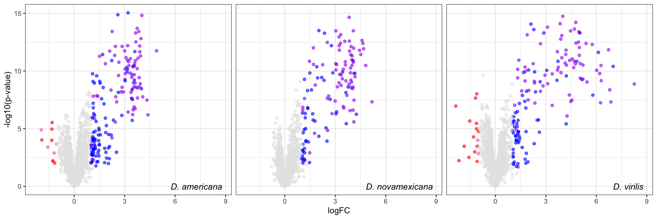
Overlap of ejaculate candidates between species
# #comb db
# upset(fromList(list(ame = comb_TABLES$Orthogroup[comb_TABLES$species == 'ame' & comb_TABLES$logFC > 1 & comb_TABLES$adj.P.Val < 0.05],
#                     nov = comb_TABLES$Orthogroup[comb_TABLES$species == 'nov' & comb_TABLES$logFC > 1 & comb_TABLES$adj.P.Val < 0.05],
#                     vir = comb_TABLES$Orthogroup[comb_TABLES$species == 'vir' & comb_TABLES$logFC > 1 & comb_TABLES$adj.P.Val < 0.05])))

#pdf('plots/sfp_overlap.pdf', height = 4, width = 4)
plot(venn(c('D. ame' = 36, "D. nov" = 7, "D. vir" = 31,
            'D. ame&D. nov' = 24, 'D. ame&D. vir' = 14, 'D. nov&D. vir' = 2,
            'D. ame&D. nov&D. vir' = 92)),
     quantities = TRUE,
     fills = list(fill = viridis::viridis(n = 3), alpha = .5))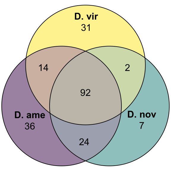
#dev.off()

# # percent overlap
# comb_TABLES %>%
#   filter(logFC > 1, adj.P.Val < 0.05) %>%
#   group_by(species) %>%
#   count() %>%
#   mutate(p = 92/n * 100)

# proportion of ejaculate candidates with signal peptide
comb_TABLES %>%
  filter(str_detect(DA, pattern = 'MB')) %>%
  distinct(genes, species, .keep_all = TRUE) %>%
  group_by(species, DA) %>% dplyr::count() %>%
  pivot_wider(id_cols = species, names_from = DA, values_from = n) %>%
  mutate(prop.sec = MBsec/(MBsec + MB)) %>%
  kable(digits = 3,
        caption = 'The number of proteins higher in abundance in mated comapred to virgin samples with or without a secretion signal for each species') %>%
kable_styling(full_width = FALSE)| species | MB | MBsec | prop.sec |
|---|---|---|---|
| ame | 90 | 76 | 0.458 |
| nov | 54 | 71 | 0.568 |
| vir | 65 | 74 | 0.532 |
Detecting artifactual differences
We look at potential differences in abundance between groups of proteins which may indicate flaws in the experimental design. For instance, ejaculate proteins may be ‘swamped out’ by the more highly abundant/speciose female reproductive tract proteins. Furthermore, serine-type endopeptidases (STEP) are down-regulated after mating - a signature of the postmating female response. If our method is effective at capturing the female reproductive tract in a ‘virgin-like’ state, then we expect no difference in the abundance of STEPs between mated and virgin samples.
Abundance of ejaculate proteins compared to remaining FRT proteins
wilc_abund <- comb_TABLES %>%
  mutate(up = if_else(adj.P.Val < 0.05 & logFC > 1, "ejac", 'frt')) %>%
  group_by(species) %>%
  do(fit = broom::tidy(wilcox.test(AveExpr ~ as.factor(up), data = .))) %>%
  unnest(fit) %>%
  mutate(up = NA,
         p.val = ifelse(p.value < 0.001, "p < 0.001", paste0('p = ', round(p.value, 3))))

comb_TABLES %>%
  mutate(up = if_else(adj.P.Val < 0.05 & logFC > 1, "Ejaculate", 'FRT')) %>%
  ggplot(aes(x = up, y = AveExpr)) +
  geom_violin(aes(fill = up), alpha = .5) +
  geom_boxplot(aes(fill = up), width = .3, notch = TRUE) +
  geom_jitter(data = comb_TABLES %>%
                mutate(up = if_else(adj.P.Val < 0.05 & logFC > 1, "Ejaculate", 'FRT')) %>%
                filter(up == 'Ejaculate'),
              colour = cbPalette[8], width = .3, alpha = .5) +
  # gghalves::geom_half_boxplot(aes(fill = up), outlier.shape = NA) +
  # gghalves::geom_half_point(aes(colour = up), alpha = .3) +
  scale_fill_manual(values = cbPalette[8:9]) +
  scale_colour_manual(values = cbPalette[8:9]) +
  facet_wrap(~species, nrow = 1, labeller = as_labeller(facet_names)) +
  labs(y = 'Average abundance') +
  theme_bw() +
  theme(legend.position = '',
        axis.title.x = element_blank(),
        strip.text = element_text(size = 15, face = "italic")) +
  geom_text(data = wilc_abund,
            aes(x = 1.5, y = 12,
                label = #paste0('Chi^2(1) = ', round(statistic, 2),
                        #       ', ',
                  p.val)) +
  # ggsignif::geom_signif(comparisons = list(c("ejac", "frt")),
  #                       map_signif_level = TRUE) +
  #ggsave('plots/ejac_vs_frt.pdf', height = 4, width = 12, dpi = 600, useDingbats = FALSE) +
  NULL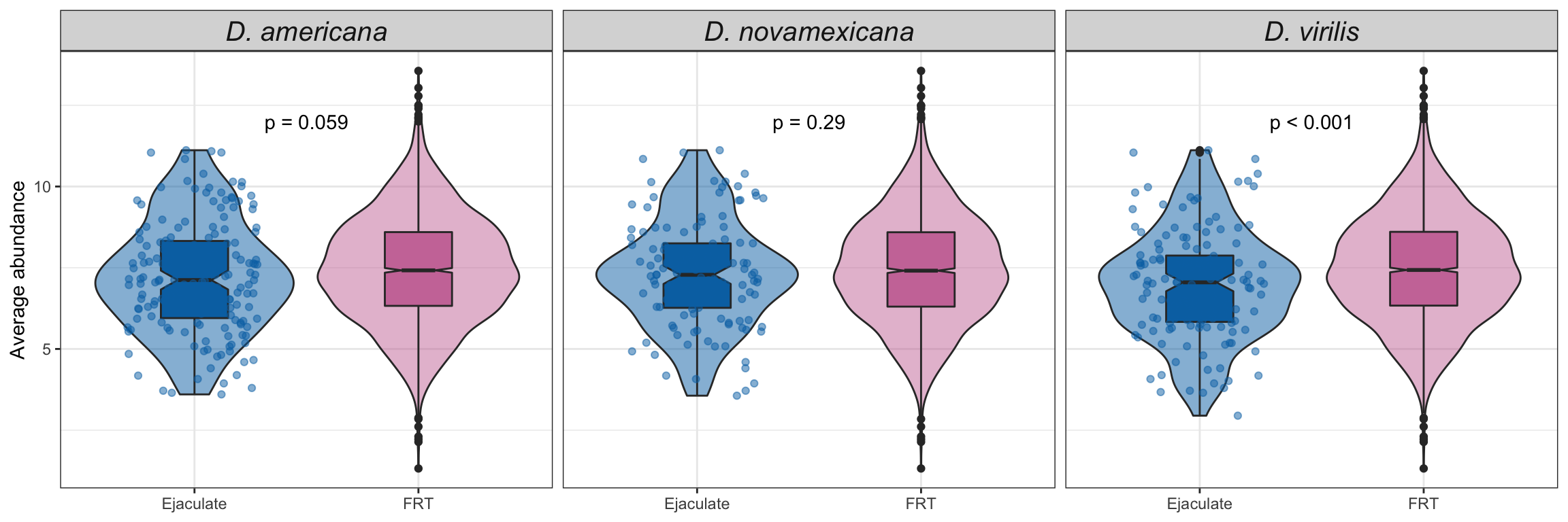
Abundance of serine-type endopeptidases
We downloaded gene ontology (GO) information for all D. virilis genes from FlyBase.org and identified all genes with serine-type endopeptidase (STEP) annotation. We tested whether these STEPs differed in abundance between samples using Kruskal-Wallis rank sum tests.
# get all genes with annotation including 'serin'
STEP <- flybase_GO %>%
  filter(stringr::str_detect(GO_BIOLOGICAL_PROCESS, 'serin') |
           stringr::str_detect(GO_MOLECULAR_FUNCTION, 'serin'))

wilc_STEP <- comb_TABLES %>%
  mutate(up = if_else(adj.P.Val < 0.05 & logFC > 1, "Ejaculate", 'FRT')) %>%
  filter(FBgn %in% STEP$FBgn) %>%
  group_by(species) %>%
  do(fit = broom::tidy(wilcox.test(AveExpr ~ as.factor(up), data = .))) %>%
  unnest(fit) %>%
  mutate(up = NA,
         p.val = ifelse(p.value < 0.001, "p < 0.001", paste0('p = ', round(p.value, 3))))

comb_TABLES %>%
  mutate(up = if_else(adj.P.Val < 0.05 & logFC > 1, "Ejaculate", 'FRT')) %>%
  filter(FBgn %in% STEP$FBgn) %>%
  ggplot(aes(x = up, y = AveExpr, fill = up)) +
  gghalves::geom_half_boxplot(aes(fill = up), outlier.shape = NA) +
  gghalves::geom_half_point(aes(colour = up), alpha = .3) +
  scale_fill_manual(values = cbPalette[8:9]) +
  scale_colour_manual(values = cbPalette[8:9]) +
  labs(y = 'Average abundance') +
  facet_wrap(~species, nrow = 1, labeller = as_labeller(facet_names)) +
  theme_bw() +
  theme(legend.position = '',
        axis.title.x = element_blank(),
        strip.text = element_text(size = 15, face = "italic")) +
  geom_text(data = wilc_STEP,
            aes(x = 1.5, y = 11,
                label = p.val)) +
  # ggsignif::geom_signif(comparisons = list(c("Ejaculate", "FRT")),
  #                       map_signif_level = TRUE) +
  #ggsave('plots/STEP_abundance.pdf', height = 3, width = 9, dpi = 600, useDingbats = FALSE) +
  NULL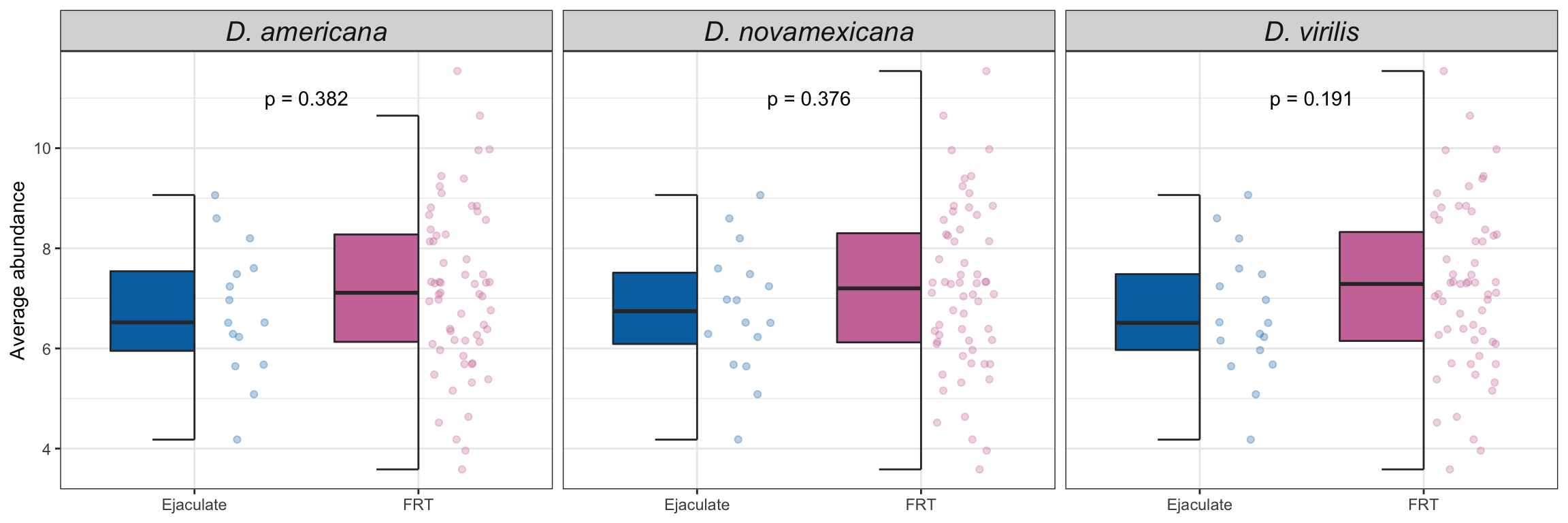
We replot the volcano plots to highlight serine-type endopeptidases, postmating female response genes and female reproductive tract genes perturbed after a heterospecific mating.
comb_TABLES %>%
  ggplot(aes(x = logFC, y = -log10(P.Value), colour = DA)) +
  geom_point() +
  scale_colour_manual(values = c('red', 'hotpink', 'blue', 'purple', 'grey90')) +
  geom_point(data = comb_TABLES %>%
    filter(threshold == 'SD' & FBgn %in% STEP$FBgn), colour = 'yellow', alpha = .3, size = 3) +
  geom_point(data = comb_TABLES %>%
    filter(threshold == 'SD' & FBgn %in% FRTbiased$FBgn_ID), colour = 'blue', alpha = .3, size = 3) +
  geom_point(data = comb_TABLES %>%
    filter(threshold == 'SD' & FBgn %in% virilisPMDE$FBgn_ID), colour = 'green', alpha = .3, size = 3) +
  facet_wrap(~species) +
  theme_bw() +
  theme(strip.text = element_text(size = 15, face = "italic")) +
  NULL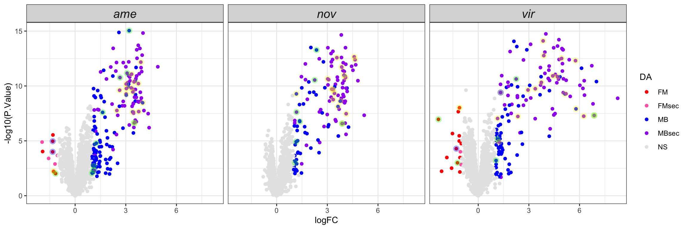
# #### Abundance of female reproductive tract biased genes and postmating female response genes
# upset(fromList(list(proteomic = comb_TABLES$FBgn,
#                     FRT_biased = FRTbiased$FBgn_ID,
#                     PMR_biased = virilisPMDE$FBgn_ID)))
#
# comb_TABLES %>% filter(FBgn %in% FRTbiased$FBgn_ID & category == 'frt')
# comb_TABLES %>% filter(FBgn %in% FRTbiased$FBgn_ID & category == 'sigFem')
#
# comb_TABLES %>% filter(FBgn %in% virilisPMDE$FBgn_ID & category == 'frt')
# comb_TABLES %>% filter(FBgn %in% virilisPMDE$FBgn_ID & category == 'sigFem')
Divergence between ejaculate candidates
We tested for differential abundance of proteins found in mated samples between each species. We restrict the data to those proteins which showed differential abundance between mated and virgin samples (adjusted p-value < 0.05 and logFC > |1|) in any species, i.e. putative male derived/Sfps/sperm proteins.
ame_cands <- ejac_cands %>% filter(DB == 'ame.db') %>%
  left_join(vir_ids) %>% distinct(Orthogroup, .keep_all = TRUE)
nov_cands <- ejac_cands %>% filter(DB == 'nov.db') %>%
  left_join(vir_ids) %>% distinct(Orthogroup, .keep_all = TRUE)
vir_cands <- ejac_cands %>% filter(DB == 'vir.db') %>%
  left_join(vir_ids) %>% distinct(Orthogroup, .keep_all = TRUE)

# # overlap between 'ejaculate candidates' identified using each species DB
# upset(fromList(list(
#   Dame = ame_cands$Orthogroup,
#   Dnov = nov_cands$Orthogroup,
#   Dvir = vir_cands$Orthogroup)))
#
# # total IDd across species
# n_distinct(na.omit(c(ame_cands$Orthogroup, nov_cands$Orthogroup, vir_cands$Orthogroup)))

# make DB
sfp_dat <- multiDB2 %>%
  filter(Orthogroup %in% c(ame_cands$Orthogroup, nov_cands$Orthogroup, vir_cands$Orthogroup)) %>%
  # remove overlap with 'female' proteins
  dplyr::select(Orthogroup, Accession_vir, contains('M'), -UP_ame) %>%
  mutate(across(3:11, ~replace_na(.x, 0)))

# make design matrix to test diffs between groups
matedSample <- sampInfo$condition[grep('M', x = sampInfo$condition)]
matedDesign <- model.matrix(~0 + matedSample)
colnames(matedDesign) <- unique(matedSample)
rownames(matedDesign) <- rep(1:3, 3)

# create DGElist and fit model
dgeSFP <- DGEList(counts = sfp_dat[, -c(1:2)], genes = sfp_dat$Accession_vir, group = matedSample)
dgeSFP <- calcNormFactors(dgeSFP, method = 'TMM')
dgeSFP <- estimateCommonDisp(dgeSFP)
dgeSFP <- estimateTagwiseDisp(dgeSFP)
# voom normalisation
dgeSFPvoom <- voom(dgeSFP, matedDesign, plot = FALSE)
# fit linear model
lmSFP <- lmFit(dgeSFPvoom, design = matedDesign)

# make contrasts - higher values = higher in first alphabetically
cont.mated <- makeContrasts(ame.MTD.nov = AM - NM,
                            ame.MTD.vir = AM - VM,
                            nov.MTD.vir = NM - VM,
                            levels = matedDesign)

# perform lmFit tests
# ame vs. nov
lm_anM <- contrasts.fit(lmSFP, cont.mated[,"ame.MTD.nov"])
lm_anM <- eBayes(lm_anM)
lm_anM.tTags.table <- topTable(lm_anM, adjust.method = "BH", number = Inf) %>%
  mutate(comparison = "aMn",
         threshold = if_else(adj.P.Val < 0.05 & abs(logFC) > 1, "SD", "NS"))

# ame vs. vir
lm_avM <- contrasts.fit(lmSFP, cont.mated[,"ame.MTD.vir"])
lm_avM <- eBayes(lm_avM)
lm_avM.tTags.table <- topTable(lm_avM, adjust.method = "BH", number = Inf) %>%
  mutate(comparison = "aMv",
         threshold = if_else(adj.P.Val < 0.05 & abs(logFC) > 1, "SD", "NS"))

# nov vs. vir
lm_nvM <- contrasts.fit(lmSFP, cont.mated[,"nov.MTD.vir"])
lm_nvM <- eBayes(lm_nvM)
lm_nvM.tTags.table <- topTable(lm_nvM, adjust.method = "BH", number = Inf) %>%
  mutate(comparison = "nMv",
         threshold = if_else(adj.P.Val < 0.05 & abs(logFC) > 1, "SD", "NS"))

mated_TABLES <- rbind(lm_anM.tTags.table,
                      lm_avM.tTags.table,
                      lm_nvM.tTags.table) %>%
  left_join(vir_ids %>% select(prot_id, FBtr, FBgn),
            by = c('genes' = 'prot_id')) %>%
  mutate(
    # add variable for signal peptides reaching significance threshold
    sigP = if_else(genes %in% c(signal_peps_ame$ID,
                                signal_peps_nov$ID,
                                signal_peps_vir$ID), 'sigP', 'not'),
    # add variable splitting by bias to virgin vs. mated and signal peptide
    sperm = if_else(FBgn %in% sperm_mel$FBgn_v, 'Sperm', 'not'),
    #Sfp = if_else(FBgn %in% wigbySFP$FBgn, 'Sfp', 'not'),
    DA = case_when(sigP == 'sigP' & threshold == 'SD' ~ "sigP",
                   threshold == 'SD' ~ "DA",
                   TRUE ~ 'NS'))

# save differentially abundant proteins to table for ClueGO
# mated_TABLES %>% filter(threshold == 'SD') %>%
#   distinct(FBgn, .keep_all = TRUE) %>% write_csv('output/ClueGOlists/Sfp_DA_multiDB.csv')
Heatmap
# make DF
sfp_md <- data.frame(dgeSFPvoom$genes,
                     dgeSFPvoom$E) %>%
  rowwise() %>%
  mutate(`D. ame` = median(c(!!! rlang::syms(grep('AM', names(.), value = TRUE)))),
         `D. nov` = median(c(!!! rlang::syms(grep('NM', names(.), value = TRUE)))),
         `D. vir` = median(c(!!! rlang::syms(grep('VM', names(.), value = TRUE))))) %>%
  #dplyr::select(genes, `D. ame`, `D. nov`, `D. vir`) %>%
  left_join(vir_ids %>% dplyr::select(prot_id, FBgn), by = c('genes' = 'prot_id')) %>%
  # add mel Sfp ortholog
  left_join(wigbySFP %>% dplyr::select(FBgn, mel_Sfp = Symbol)) %>%
  mutate(category = case_when(genes %in% sperm_mel$prot_id ~ 'sperm',
                              FBgn %in% wigbySFP$FBgn ~ 'Sfp',
                              genes %in% vir_sig$ID ~ 'sigP',
                              TRUE ~ 'other'))

sfp_hm <- sfp_md %>%
  dplyr::select(`D. ame`, `D. nov`, `D. vir`,
                FBgn, mel_Sfp, category)

row.names(sfp_hm) <- sfp_md$genes

mat_scaled <- t(apply(sfp_hm[, 1:3], 1, scale))

library(cluster)
library(factoextra)

# Dissimilarity matrix
d <- dist(mat_scaled, method = "euclidean")

# Hierarchical clustering using Complete Linkage
hc1 <- hclust(d, method = "complete" )

# Plot the obtained dendrogram
#plot(hc1, cex = 0.6, hang = -1)

fviz_nbclust(mat_scaled, FUN = hcut, method = "silhouette")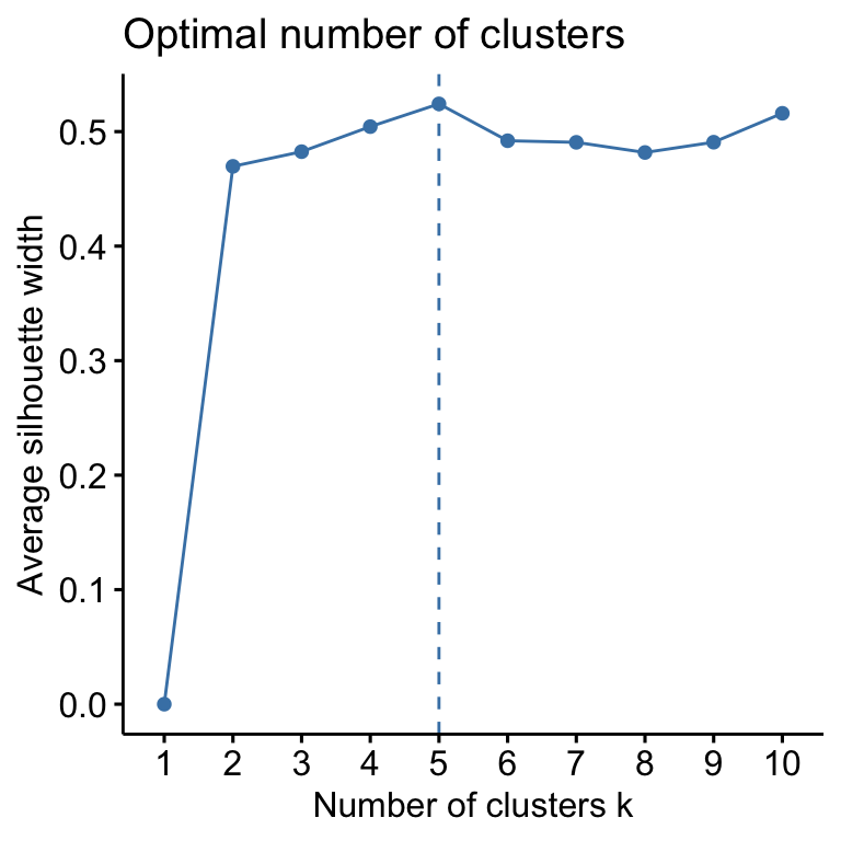
# Cut tree into 5 groups
sub_grp <- cutree(hc1, k = 5)

# heatmap annotations
cat_lab <- rowAnnotation(Cluster = sub_grp,
                         col = list(Cluster = setNames(cbPalette[2:6], unique(sub_grp))),
                         title = NULL,
                         show_annotation_name = FALSE)

Sfp_labs <- rowAnnotation(Category = sfp_md$category,
                          col = list(Category = c(sperm = v.pal[2],
                                                  Sfp = v.pal[3],
                                                  sigP = v.pal[1],
                                                  other = NA)),
                          Sfp_labs = anno_mark(at = c(grep('Sfp', x = sfp_md$category)),
                                               labels = sfp_md$mel_Sfp[sfp_md$category == 'Sfp'],
                                               labels_gp = gpar(fontsize = 8)),
                          title = NULL,
                          show_annotation_name = FALSE)

haha <- HeatmapAnnotation(species = anno_block(gp = gpar(fill = c(v.pal[c(1, 3, 2)])),
                                               labels = c(expression(italic('D. vir')),
                                                          expression(italic('D. ame')),
                                                          expression(italic('D. nov'))),
                                               labels_gp = gpar(col = c('black', 'white', 'white'),
                                                                fontsize = 10)))

sfp_chm <- Heatmap(mat_scaled,
                   col = viridis::inferno(100),
                   heatmap_legend_param = list(title = "log2(intensities)",
                                               title_position = "leftcenter-rot"),
                   right_annotation = Sfp_labs,
                   left_annotation = cat_lab,
                   top_annotation = haha,
                   show_row_names = FALSE,
                   show_column_names = FALSE,
                   row_split = 5,
                   column_split = 3,
                   column_gap = unit(0, "mm"),
                   row_title = NULL,
                   column_title = NULL)
#pdf('plots/sfp_compheatmap.pdf', height = 8, width = 5)
sfp_chm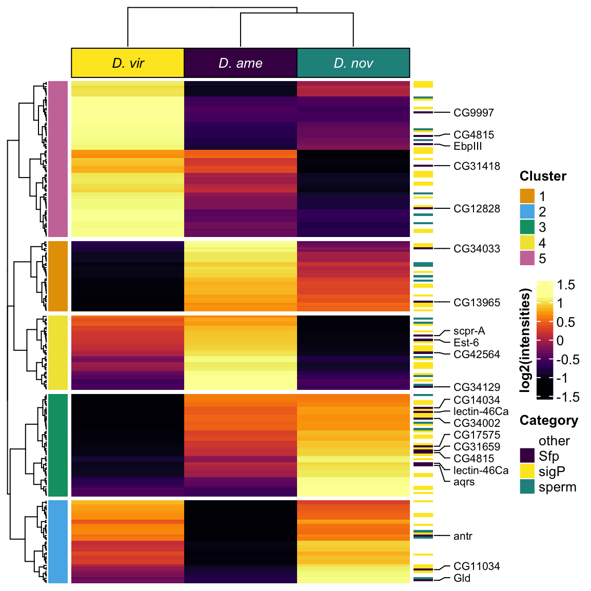
#dev.off()We tested how protein abundance differed between species based on k-means cluster
sfp_cluster <- sfp_md %>%
  dplyr::select(genes, FBgn, 11:13) %>%
  bind_cols(cluster = sub_grp) %>%
  pivot_longer(cols = 3:5) %>%
  mutate(species = str_sub(name, 4, 4))

sfp_cluster %>%
  mutate(cluster = paste('Cluster', cluster, sep = ' ')) %>%
  ggplot(aes(x = factor(name, levels = c('D. vir', 'D. ame', 'D. nov')), y = value, fill = name)) +
  gghalves::geom_half_point(aes(colour = name)) +
  gghalves::geom_half_violin(aes(fill = name)) +
  stat_pointinterval(pch = 21, fill = 'white') +
  labs(x = 'Species', y = 'normalised abundance') +
  scale_fill_viridis_d() +
  scale_colour_viridis_d() +
  facet_wrap(~cluster, scales = 'free_y') +
  theme_bw() +
  theme(legend.position = '',
        axis.text.x = element_text(face = 'italic')) +
  ggpubr::stat_compare_means(aes(label = ..p.signif..),
                             comparisons = list(c('D. ame', 'D. nov'),
                                                c('D. ame', 'D. vir'),
                                                c('D. nov', 'D. vir')),
                             method = 't.test') +
  #ggsave('plots/sfp_pointinterval.pdf', height = 4, width = 6, dpi = 600, useDingbats = FALSE) +
  NULL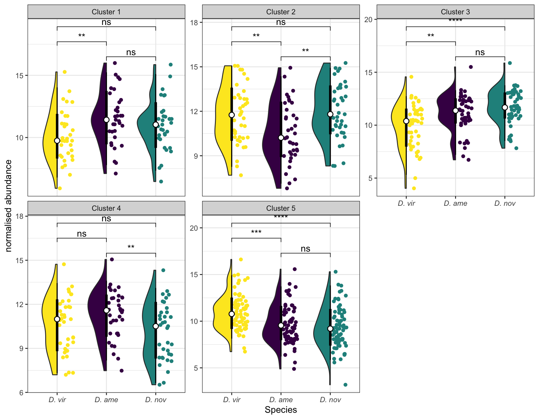
Diagnostic plots
residual vs. fitted
sfp_cluster %>% group_by(cluster) %>%
  do(fit = broom::augment(lm(value ~ name, data = .))) %>%
  unnest(fit) %>%
  ggplot(aes(x = .fitted, y = .std.resid)) +
  geom_point() +
  geom_smooth(colour = 'red', se = FALSE) +
  facet_wrap(~cluster, scales = 'free')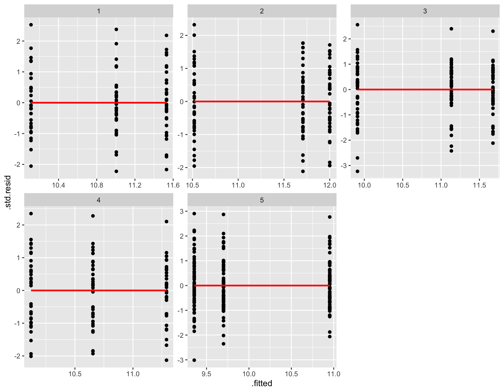
| Version | Author | Date |
|---|---|---|
| f28e7a0 | MartinGarlovsky | 2022-02-07 |
Scale location
sfp_cluster %>% group_by(cluster) %>%
  do(fit = broom::augment(lm(value ~ name, data = .))) %>%
  unnest(fit) %>%
  ggplot(aes(x = .fitted, y = sqrt(abs(.std.resid)))) +
  geom_point() +
  geom_smooth(colour = 'red', se = FALSE) +
  facet_wrap(~cluster, scales = 'free')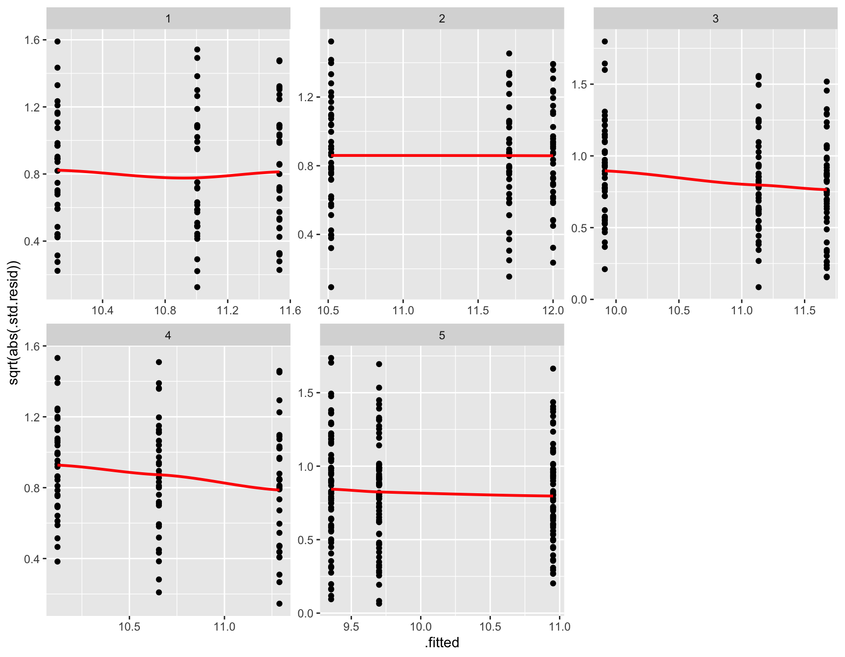
QQ plot
sfp_cluster %>% group_by(cluster) %>%
  do(fit = broom::augment(lm(value ~ name, data = .))) %>%
  unnest(fit) %>%
  ggplot(aes(sample = .std.resid)) +
  stat_qq() + geom_abline(slope = 1) +
  facet_wrap(~cluster, scales = 'free')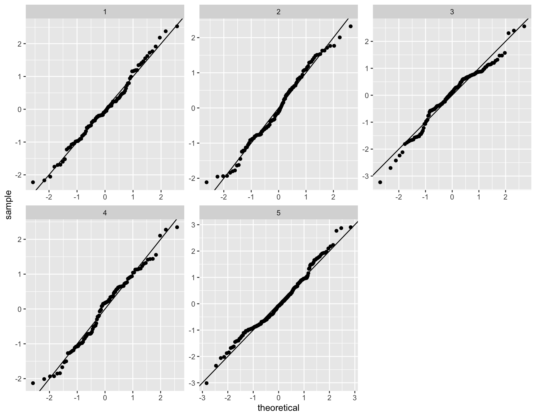
Residuals vs leverage
sfp_cluster %>% group_by(cluster) %>%
  do(fit = broom::augment(lm(value ~ name, data = .))) %>%
  unnest(fit) %>%
  ggplot(aes(x = .std.resid, y = .hat)) +
  geom_point() +
  geom_smooth(colour = 'red', se = FALSE) +
  facet_wrap(~cluster, scales = 'free')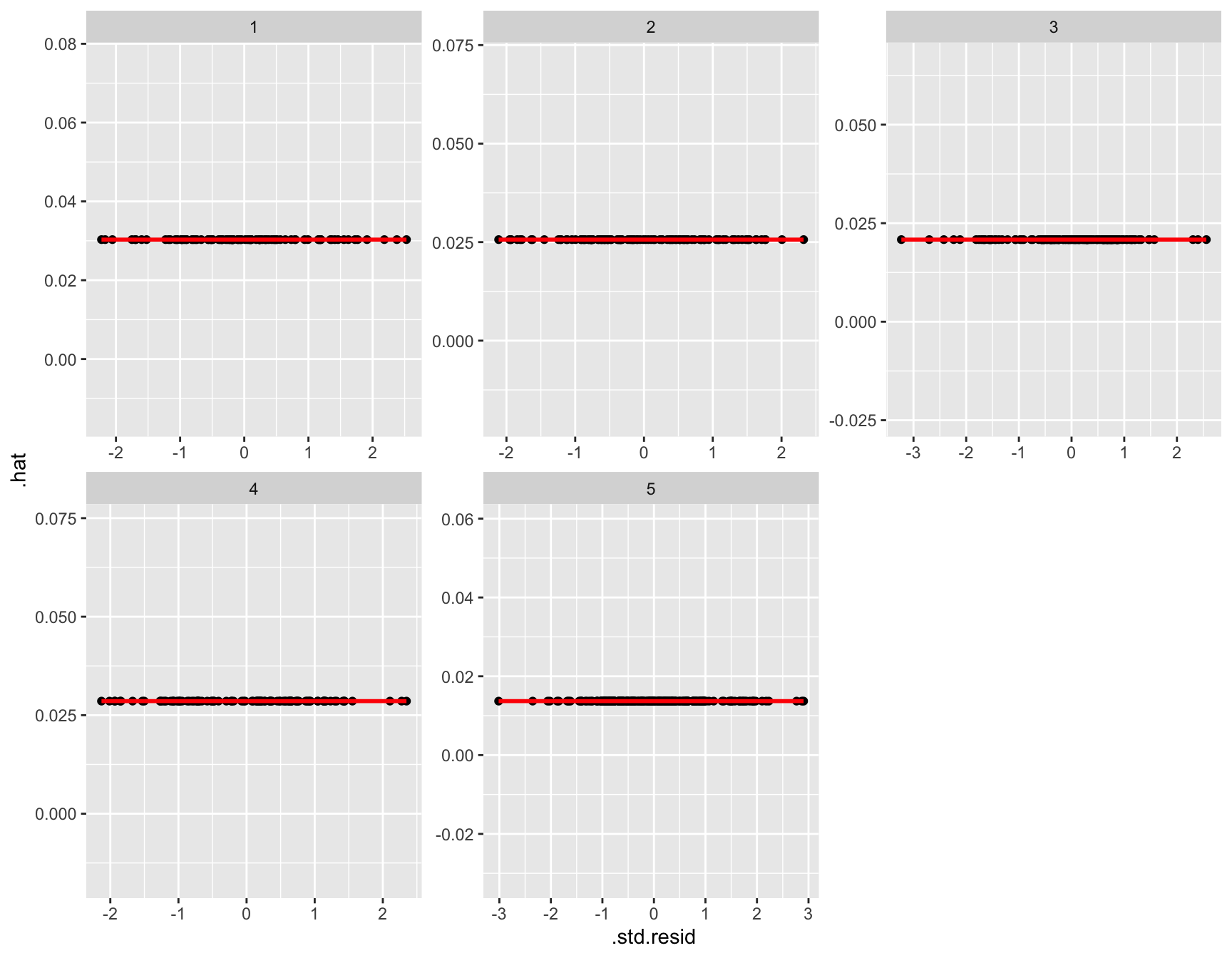
Model fits
sfp_cluster %>% group_by(cluster) %>%
  do(fit = broom::glance(lm(value ~ name, data = .))) %>%
  unnest(fit) %>%
  mutate(p.value = ifelse(p.value < 0.001, '< 0.001', round(p.value, 3))) %>%
  dplyr::select(-adj.r.squared, -sigma, -c(df:nobs)) %>%
  kable(digits = 3,
        caption = 'Model fits') %>%
kable_styling(full_width = FALSE)| cluster | r.squared | statistic | p.value |
|---|---|---|---|
| 1 | 0.076 | 3.948 | 0.022 |
| 2 | 0.102 | 6.456 | 0.002 |
| 3 | 0.141 | 11.602 | < 0.001 |
| 4 | 0.066 | 3.631 | 0.03 |
| 5 | 0.101 | 12.168 | < 0.001 |
sfp_cluster %>% group_by(cluster) %>%
  do(fit = broom::tidy(lm(value ~ name, data = .))) %>%
  unnest(fit) %>%
  mutate(p.value = ifelse(p.value < 0.001, '< 0.001', round(p.value, 3)),
         sigLabel = case_when(p.value < 0.001 ~ "***",
                              p.value < 0.01 ~ "**",
                              p.value < 0.05 ~ "*",
                              TRUE ~ '')) %>%
  kable(digits = 3,
        caption = 'Model estimates') %>%
kable_styling(full_width = FALSE)| cluster | term | estimate | std.error | statistic | p.value | sigLabel |
|---|---|---|---|---|---|---|
| 1 | (Intercept) | 11.531 | 0.361 | 31.937 | < 0.001 | *** |
| 1 | nameD. nov | -0.525 | 0.511 | -1.029 | 0.306 | |
| 1 | nameD. vir | -1.419 | 0.511 | -2.779 | 0.007 | ** |
| 2 | (Intercept) | 10.520 | 0.309 | 34.095 | < 0.001 | *** |
| 2 | nameD. nov | 1.480 | 0.436 | 3.393 | < 0.001 | *** |
| 2 | nameD. vir | 1.188 | 0.436 | 2.721 | 0.008 | ** |
| 3 | (Intercept) | 11.134 | 0.266 | 41.936 | < 0.001 | *** |
| 3 | nameD. nov | 0.542 | 0.375 | 1.443 | 0.151 | |
| 3 | nameD. vir | -1.224 | 0.375 | -3.259 | 0.001 | ** |
| 4 | (Intercept) | 11.289 | 0.307 | 36.794 | < 0.001 | *** |
| 4 | nameD. nov | -1.168 | 0.434 | -2.692 | 0.008 | ** |
| 4 | nameD. vir | -0.634 | 0.434 | -1.461 | 0.147 | |
| 5 | (Intercept) | 9.700 | 0.241 | 40.247 | < 0.001 | *** |
| 5 | nameD. nov | -0.345 | 0.341 | -1.013 | 0.312 | |
| 5 | nameD. vir | 1.253 | 0.341 | 3.675 | < 0.001 | *** |
sfp_cluster %>% group_by(cluster) %>%
  do(fit = broom::tidy(TukeyHSD(aov(value ~ name, data = .)))) %>%
  unnest(fit) %>%
  mutate(contrast = recode(contrast,
                      `D. nov-D. ame` = "D. ame vs. D. nov",
                      `D. vir-D. ame` = "D. ame vs. D. vir",
                      `D. vir-D. nov` = 'D. nov vs. D. vir'),
         p.value = ifelse(adj.p.value < 0.001, '< 0.001', round(adj.p.value, 3)),
         across(4:8, ~ round(.x, 2)),
         Estimate = paste0(estimate, ' (', conf.low, '-', conf.high, ')'),
         sigLabel = case_when(p.value < 0.001 ~ "***",
                              p.value < 0.01 ~ "**",
                              p.value < 0.05 ~ "*",
                              TRUE ~ '')) %>%
  dplyr::select(-term, -null.value, -c(estimate:adj.p.value)) %>%
  kable(digits = 3,
        caption = 'Post hoc contrasts') %>%
kable_styling(full_width = FALSE)| cluster | contrast | p.value | Estimate | sigLabel |
|---|---|---|---|---|
| 1 | D. ame vs. D. nov | 0.56 | -0.53 (-1.74-0.69) | |
| 1 | D. ame vs. D. vir | 0.018 | -1.42 (-2.63–0.2) |
|
| 1 | D. nov vs. D. vir | 0.192 | -0.89 (-2.11-0.32) | |
| 2 | D. ame vs. D. nov | 0.003 | 1.48 (0.44-2.52) | ** |
| 2 | D. ame vs. D. vir | 0.02 | 1.19 (0.15-2.22) |
|
| 2 | D. nov vs. D. vir | 0.781 | -0.29 (-1.33-0.74) | |
| 3 | D. ame vs. D. nov | 0.322 | 0.54 (-0.35-1.43) | |
| 3 | D. ame vs. D. vir | 0.004 | -1.22 (-2.11–0.33) | ** |
| 3 | D. nov vs. D. vir | < 0.001 | -1.77 (-2.65–0.88) | *** |
| 4 | D. ame vs. D. nov | 0.022 | -1.17 (-2.2–0.14) |
|
| 4 | D. ame vs. D. vir | 0.314 | -0.63 (-1.67-0.4) | |
| 4 | D. nov vs. D. vir | 0.438 | 0.53 (-0.5-1.57) | |
| 5 | D. ame vs. D. nov | 0.57 | -0.35 (-1.15-0.46) | |
| 5 | D. ame vs. D. vir | < 0.001 | 1.25 (0.45-2.06) | *** |
| 5 | D. nov vs. D. vir | < 0.001 | 1.6 (0.79-2.4) | *** |
Volcano plots
mated_TABLES %>% filter(DA != 'NS') %>%
  ggplot(aes(x = logFC, y = -log10(P.Value), colour = DA)) +
  geom_point(data = mated_TABLES %>% filter(DA == 'NS'), colour = 'grey') +
  geom_point(alpha = .6) +
  #scale_colour_manual(values = c('hotpink', 'red', 'blue')) +
  labs(y = '-log10(p-value)') +
  facet_wrap(~comparison, nrow = 1,
             labeller = as_labeller(c(aMn = "D. americana vs. D. novamexicana",
                                      aMv = 'D. americana vs. D. virilis',
                                      nMv = "D. novamexicana vs. D. virilis"))) +
  theme_bw() +
  theme(legend.position = c(0.04, 0.2),
        legend.background = element_rect(fill = NA),
        legend.title = element_blank(),
        strip.text = element_text(size = 15, face = "italic")) +
  geom_label_repel(
    data = mated_TABLES %>% filter(DA != 'NS') %>% left_join(wigbySFP, by = 'FBgn'),
    aes(label = Symbol),
    size = 4,
    colour = 'black',
    box.padding = unit(0.35, "lines"),
    point.padding = unit(0.3, "lines")
  ) +
  #ggsave('plots/volcano_sfp.pdf', height = 4, width = 12, dpi = 600, useDingbats = FALSE) +
  NULL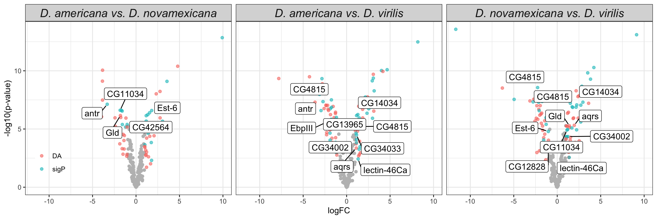
# # wigby Sfps IDd as DA in each comparison
# mated_TABLES %>% filter(DA != 'NS') %>%
#   left_join(wigbySFP, by = 'FBgn') %>%
#   filter(comparison == 'aMn') %>% drop_na(Symbol)
#
# mated_TABLES %>% filter(DA != 'NS') %>%
#   left_join(wigbySFP, by = 'FBgn') %>%
#   filter(comparison == 'aMv') %>% drop_na(Symbol)
#
# mated_TABLES %>% filter(DA != 'NS') %>%
#   left_join(wigbySFP, by = 'FBgn') %>%
#   filter(comparison == 'nMv') %>% drop_na(Symbol)
Are signal peps more likely to be DA?
mated_TABLES %>%
  group_by(comparison, threshold, sigP) %>% dplyr::count() %>%
  ggplot(aes(x = threshold, y = n, fill = sigP)) +
  geom_col(position = 'fill') +
  facet_wrap(~comparison, nrow = 1,
             labeller = as_labeller(c(aMn = "D. americana vs. D. novamexicana",
                                      aMv = 'D. americana vs. D. virilis',
                                      nMv = "D. novamexicana vs. D. virilis"))) +
  theme_bw() +
  NULL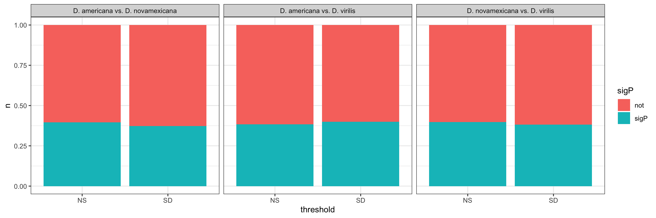
# Fisher's exact tests
mated_TABLES %>%
  group_by(comparison) %>%
  do(fit = broom::tidy(fisher.test(as.matrix(xtabs(~ threshold + sigP, ., sparse = T))))) %>%
  unnest(fit) %>%
  mutate(comparison = recode(comparison,
                             aMn = "D. ame vs. D. nov",
                             aMv = "D. ame vs. D. vir",
                             nMv = 'D. nov vs. D. vir'),
         across(2:5, ~ round(.x, 2)),
         p.value = ifelse(p.value < 0.001, "< 0.001", p.value),
         Estimate = paste0(estimate, ' (', conf.low, '-', conf.high, ')')) %>%
  dplyr::select(Comparison = comparison, Estimate, p.value) %>%
  kable(caption = 'Fisher\'s exact tests for signal peptides that are differentially abundant or not') %>%
kable_styling(full_width = FALSE)| Comparison | Estimate | p.value |
|---|---|---|
| D. ame vs. D. nov | 0.91 (0.47-1.73) | 0.88 |
| D. ame vs. D. vir | 1.07 (0.61-1.9) | 0.89 |
| D. nov vs. D. vir | 0.94 (0.53-1.66) | 0.89 |
# are sperm genes more likely to be DA?
mated_TABLES %>%
  #filter(sperm == 'Sperm') %>%
  group_by(comparison, threshold, sperm) %>% dplyr::count() %>%
  ggplot(aes(x = sperm, y = n, fill = threshold)) +
  geom_col(position = 'fill') +
  facet_wrap(~comparison, nrow = 1,
             labeller = as_labeller(c(aMn = "D. americana vs. D. novamexicana",
                                      aMv = 'D. americana vs. D. virilis',
                                      nMv = "D. novamexicana vs. D. virilis"))) +
  theme_bw() +
  theme(strip.text = element_text(size = 15, face = "italic")) +
  NULL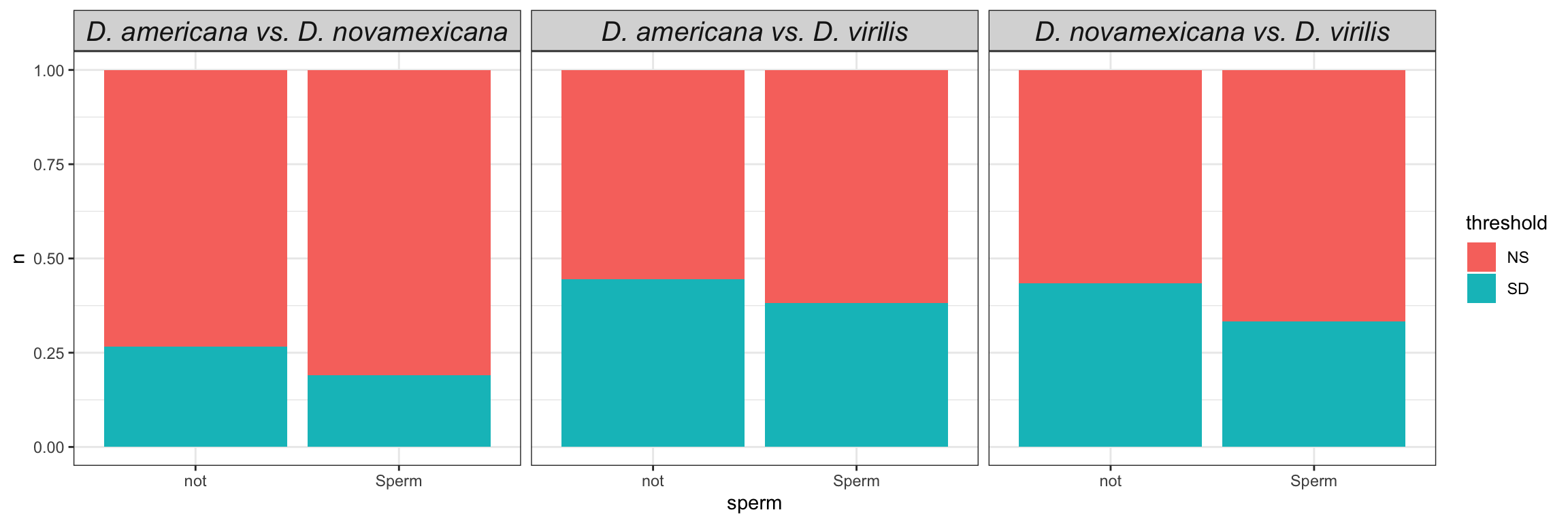
# Fisher's exact tests
mated_TABLES %>%
  group_by(comparison) %>%
  do(fit = broom::tidy(fisher.test(as.matrix(xtabs(~ threshold + sperm, ., sparse = T))))) %>%
  unnest(fit) %>%
  mutate(across(2:5, ~ round(.x, 2)),
         p.value = ifelse(p.value < 0.001, '< 0.001', round(p.value, 3)),
         Estimate = paste0(estimate, ' (', conf.low, '-', conf.high, ')')) %>%
  dplyr::select(comparison, Estimate, p.value) %>%
  kable(digits = 3,
        caption = 'Fisher\'s exact tests for sperm proteins that are differentially abundant or not') %>%
kable_styling(full_width = FALSE)| comparison | Estimate | p.value |
|---|---|---|
| aMn | 0.65 (0.15-2.12) | 0.60 |
| aMv | 0.77 (0.26-2.1) | 0.65 |
| nMv | 0.65 (0.21-1.81) | 0.49 |
Overlap between DA proteins
# upset(fromList(list(
#   a.vs.n = lm_anM.tTags.table$genes[lm_anM.tTags.table$threshold == 'SD'],
#   a.vs.v = lm_avM.tTags.table$genes[lm_avM.tTags.table$threshold == 'SD'],
#   n.vs.v = lm_nvM.tTags.table$genes[lm_nvM.tTags.table$threshold == 'SD'])))

#pdf('plots/divergence_overlap_comb.pdf', height = 4, width = 4)
plot(euler(c('a.vs.n' = 12, 'a.vs.v' = 10, 'n.vs.v' = 11,
             'a.vs.n&a.vs.v' = 20, 'a.vs.n&n.vs.v' = 16, 'a.vs.v&n.vs.v' = 59,
             'a.vs.n&a.vs.v&n.vs.v' = 11)),
     quantities = TRUE,
     fills = list(fill = cbPalette[2:4], alpha = .5))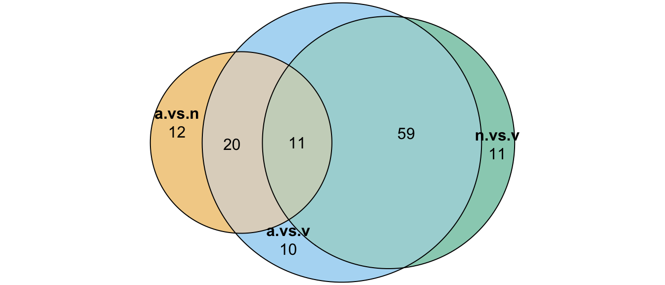
#dev.off()Divergence between (virgin) reproductive tracts
fem_dat <- multiDB2 %>%
  filter(!Orthogroup %in% c(ame_cands$Orthogroup, nov_cands$Orthogroup, vir_cands$Orthogroup)) %>%
  dplyr::select(-contains('M'), -contains('UP_')) %>%
  mutate(across(4:10, ~replace_na(.x, 0)))

# # most identified sperm proteins remain in virgin samples after excluding DA proteins between mated/viring samples
# fem_dat %>%
#   filter(Accession_vir %in% sperm_mel$prot_id)

# make design matrix to test diffs between groups
femSample <- sampInfo$condition[grep('V$', x = sampInfo$condition)]
femdesign <- model.matrix(~0 + femSample)
colnames(femdesign) <- unique(femSample)
rownames(femdesign) <- c(rep(1:2, 2), 1:3)

# create DGElist and fit model
dgeFEM <- DGEList(counts = fem_dat[, -c(1:3)], genes = fem_dat$Accession_vir, group = femSample)
dgeFEM <- calcNormFactors(dgeFEM, method = 'TMM')
dgeFEM <- estimateCommonDisp(dgeFEM)
dgeFEM <- estimateTagwiseDisp(dgeFEM)
# voom normalisation
dgeFEMvoom <- voom(dgeFEM, femdesign, plot = FALSE)
# fit linear model
lmFEM <- lmFit(dgeFEMvoom, design = femdesign)

# make contrasts - higher values = higher in first alphabetically
cont.fem <- makeContrasts(ame.FEM.nov = AV - NV,
                          ame.FEM.vir = AV - VV,
                          nov.FEM.vir = NV - VV,
                          levels = femdesign)

# perform lmFit tests
# ame vs. nov
lm_anF <- contrasts.fit(lmFEM, cont.fem[,"ame.FEM.nov"])
lm_anF <- eBayes(lm_anF)
lm_anF.tTags.table <- topTable(lm_anF, adjust.method = "BH", number = Inf) %>%
  mutate(comparison = "aVn",
         threshold = if_else(adj.P.Val < 0.05 & abs(logFC) > 1, "SD", "NS"))

# ame vs. vir
lm_avF <- contrasts.fit(lmFEM, cont.fem[,"ame.FEM.vir"])
lm_avF <- eBayes(lm_avF)
lm_avF.tTags.table <- topTable(lm_avF, adjust.method = "BH", number = Inf) %>%
  mutate(comparison = "aVv",
         threshold = if_else(adj.P.Val < 0.05 & abs(logFC) > 1, "SD", "NS"))

# nov vs. vir
lm_nvF <- contrasts.fit(lmFEM, cont.fem[,"nov.FEM.vir"])
lm_nvF <- eBayes(lm_nvF)
lm_nvF.tTags.table <- topTable(lm_nvF, adjust.method = "BH", number = Inf) %>%
  mutate(comparison = "nVv",
         threshold = if_else(adj.P.Val < 0.05 & abs(logFC) > 1, "SD", "NS"))

fem_TABLES <- rbind(lm_anF.tTags.table,
                    lm_avF.tTags.table,
                    lm_nvF.tTags.table) %>%
  left_join(fem_dat,
            by = c('genes' = 'Accession_vir')) %>%
   mutate(
    # add variable for signal peptides reaching significance threshold
    sigP = if_else(genes %in% c(signal_peps_ame$ID,
                                signal_peps_nov$ID,
                                signal_peps_vir$ID), 'sigP', 'not'),
    spec = case_when(FBgn %in% virilisPMDE$FBgn_ID ~ 'PMR',
                     FBgn %in% FRTbiased$FBgn_ID ~ 'FRT',
                     genes %in% c(signal_peps_ame$ID,
                                  signal_peps_nov$ID,
                                  signal_peps_vir$ID) & threshold == 'SD' ~ 'sigP',
                     TRUE ~ 'other'))

# # numbers of differentially abundant...
# # PMR proteins
# fem_TABLES %>% filter(FBgn %in% virilisPMDE$FBgn_ID & threshold == 'SD') %>%
#   group_by(comparison) %>% count()
#
# # FRT proteins
# fem_TABLES %>% filter(FBgn %in% FRTbiased$FBgn_ID & threshold == 'SD') %>%
#   group_by(comparison) %>% count()
#
# # signal peptides
# fem_TABLES %>% filter(genes %in% c(signal_peps_ame$ID,
#                                    signal_peps_nov$ID,
#                                    signal_peps_vir$ID) & threshold == 'SD') %>%
#   group_by(comparison) %>% count()
Are signal peps more likely to be DA?
# are signal peps more likely to be DA?
fem_TABLES %>%
  group_by(comparison, threshold, sigP) %>% dplyr::count() %>%
  ggplot(aes(x = threshold, y = n, fill = sigP)) +
  geom_col(position = 'fill') +
  facet_wrap(~comparison, nrow = 1,
             labeller = as_labeller(c(aVn = "D. americana vs. D. novamexicana",
                                      aVv = 'D. americana vs. D. virilis',
                                      nVv = "D. novamexicana vs. D. virilis"))) +
  theme_bw() +
  NULL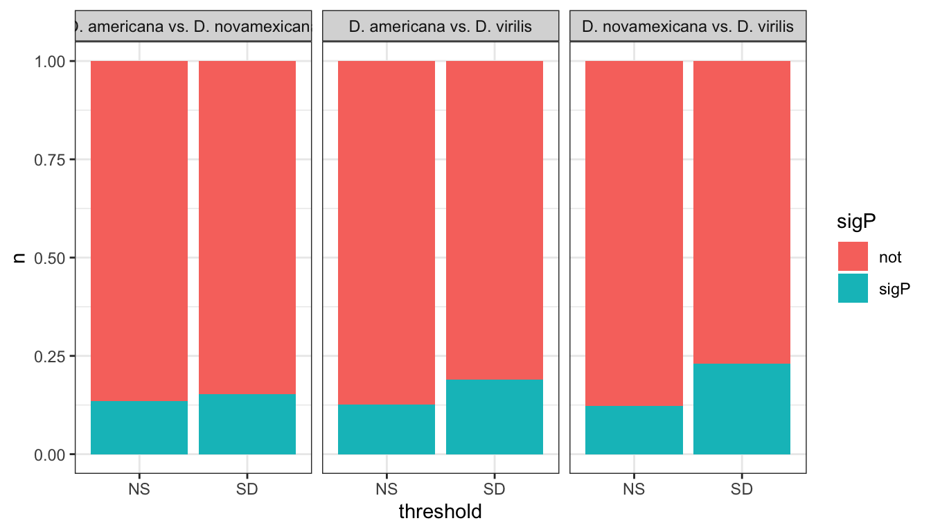
# Fisher's exact tests
# Model fits
fem_TABLES %>% group_by(comparison) %>%
  do(fit = broom::glance(fisher.test(as.matrix(xtabs(~ threshold + sigP, ., sparse = T))))) %>%
  unnest(fit) %>%
  mutate(across(2:5, ~ round(.x, 2)),
         p.value = ifelse(p.value < 0.001, '< 0.001', round(p.value, 3)),
         comparison = recode(comparison,
                             aVn = "D. ame vs. D. nov", aVv = "D. ame vs. D. vir", nVv = 'D. nov vs. D. vir'),
         Estimate = paste0(estimate, ' (', conf.low, '-', conf.high, ')')) %>%
  dplyr::select(comparison, Estimate, p.value) %>%
  kable(caption = 'Proportion of signal peptides showing differential abundance between species. Fisher\'s exact tests') %>%
kable_styling(full_width = FALSE)| comparison | Estimate | p.value |
|---|---|---|
| D. ame vs. D. nov | 1.15 (0.81-1.61) | 0.39 |
| D. ame vs. D. vir | 1.62 (1.22-2.13) | < 0.001 |
| D. nov vs. D. vir | 2.14 (1.59-2.85) | < 0.001 |
# #save proteins minus ejaculate candidates i.e. remaining proteins as 'female'
# fem_TABLES %>%
#   filter(!FBgn %in% ejac_cands$FBgn) %>%
#   distinct(FBgn, .keep_all = TRUE) %>%
#   write_csv('output/ClueGOlists/all_NOTejac_FBgn.csv')

# #save proteins minus ejaculate candidates i.e. remaining proteins as 'female' & signal pep
# fem_TABLES %>%
#   filter(!FBgn %in% ejac_cands$FBgn) %>%
#   filter(sigP == 'sigP') %>%
#   distinct(FBgn, .keep_all = TRUE) %>%
#   write_csv('output/ClueGOlists/all_frtSigP_FBgn.csv')

# save differentially abundant proteins to table for ClueGO
# fem_TABLES %>% filter(threshold == 'SD') %>%
#   distinct(FBgn, .keep_all = TRUE) %>% write_csv('output/ClueGOlists/virgin_DA_multiDB.csv')
Volcano plots
fem_TABLES %>%
  ggplot(aes(x = logFC, y = -log10(P.Value), colour = spec)) +
  geom_point(data = fem_TABLES %>% filter(threshold == 'NS'), shape = 1, alpha = .1, colour = 'grey') +
  geom_point(alpha = .5) +
  scale_colour_brewer(palette = 'RdBu') +
  #scale_colour_viridis_d(option = 'C') +
  labs(y = '-log10(p-value)') +
  facet_wrap(~comparison, nrow = 1,
             labeller = as_labeller(c(aVn = "D. americana vs. D. novamexicana",
                                      aVv = 'D. americana vs. D. virilis',
                                      nVv = "D. novamexicana vs. D. virilis"))) +
  theme_bw() +
  theme(legend.position = c(0.04, 0.2),
        legend.title = element_blank(),
        legend.background = element_rect(fill = NA),
        strip.text = element_text(size = 15, face = "italic")) +
  #ggsave('plots/volcano_FRTbtSp.pdf', height = 4, width = 12, dpi = 600, useDingbats = FALSE) +
  NULL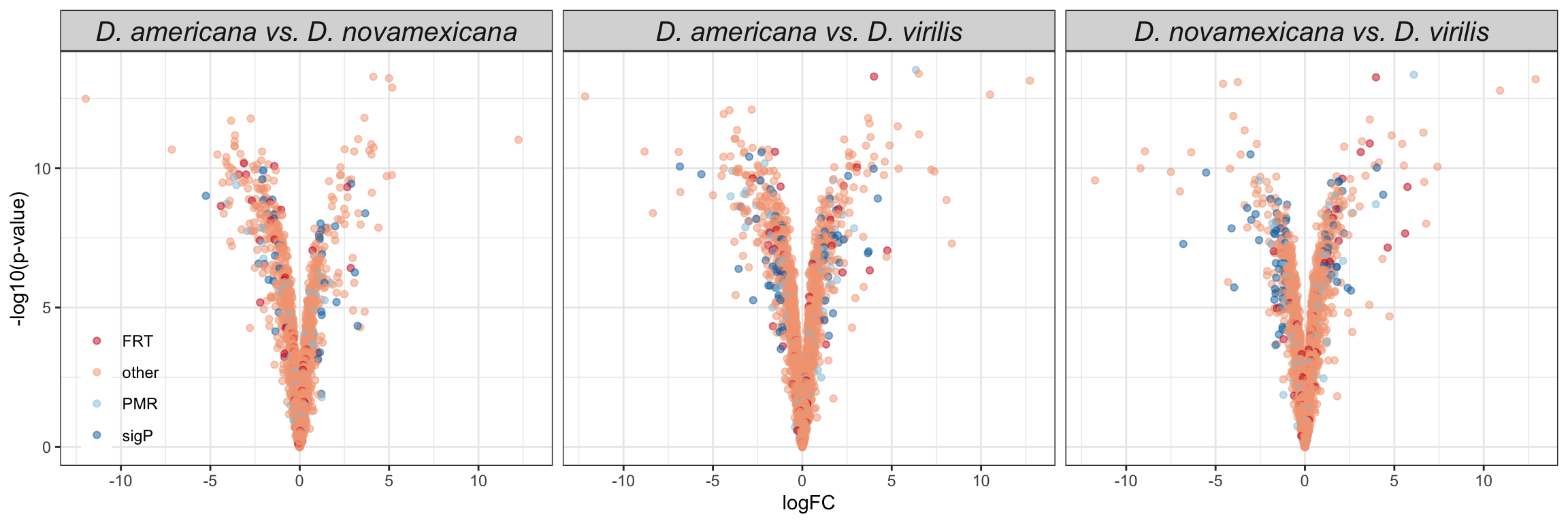
Heatmap
All proteins
fem_md <- data.frame(dgeFEMvoom$genes,
                     dgeFEMvoom$E) %>%
  rowwise() %>%
  mutate(`D. ame` = median(c(!!! rlang::syms(grep('A', names(.), value = TRUE)))),
         `D. nov` = median(c(!!! rlang::syms(grep('NV', names(.), value = TRUE)))),
         `D. vir` = median(c(!!! rlang::syms(grep('VV', names(.), value = TRUE))))) %>%
  left_join(vir_ids, by = c('genes' = 'prot_id')) %>%
  mutate(Ejac = ifelse(genes %in% c(ame_cands$Accession_vir,
                                    nov_cands$Accession_vir,
                                    vir_cands$Accession_vir), 'Ejac', NA),
         category = case_when(genes %in% sperm_mel$prot_id ~ 'sperm',
                              FBgn %in% wigbySFP$FBgn ~ 'Sfp',
                              TRUE ~ as.character(NA)),
         fem_cat = case_when(FBgn %in% STEP$FBgn ~ 'STEP',
                             FBgn %in% FRTbiased$FBgn_ID ~ 'FRT',
                             FBgn %in% virilisPMDE$FBgn_ID ~ 'pmr',
                             genes %in% vir_sig$ID ~ 'sig',
                             TRUE ~ as.character(NA))) %>%
  left_join(flybase_GO %>% dplyr::select(FBgn, Symbol = mel_GeneSymbol), by = 'FBgn') %>%
  mutate(Symbol = if_else(is.na(Symbol), FBgn, Symbol))

# scale data
mat_scaled_frt <- t(apply(fem_md[, 9:11], 1, scale))

# Dissimilarity matrix
df <- dist(mat_scaled_frt, method = "euclidean")

# Hierarchical clustering using Complete Linkage
hc1f <- hclust(df, method = "complete" )

# Plot the dendrogram
#plot(hc1, cex = 0.6, hang = -1)

#fviz_nbclust(mat_scaled_frt, FUN = hcut, method = "silhouette")

# Cut tree into 6 groups
sub_grpf <- cutree(hc1f, k = 6)

# Number of members in each cluster
#table(sub_grpf)

cat_lab <- rowAnnotation(clust_lab = sub_grpf,
                         col = list(clust_lab = setNames(cbPalette[2:7], unique(sub_grpf))),
                         title = NULL,
                         show_annotation_name = FALSE)

frt_lab <- rowAnnotation(Category = fem_md$fem_cat,
                         col = list(Category = setNames(c('chocolate', 'orange', 'hotpink', 'cyan'),
                                                        unique(na.omit(fem_md$fem_cat)))),
                         frt_labs = anno_mark(at = c(grep('STEP', x = fem_md$fem_cat)),
                                              labels = na.omit(fem_md$Symbol[fem_md$fem_cat == 'STEP']),
                                              labels_gp = gpar(fontsize = 8)),
                         title = NULL,
                         na_col = NA,
                         show_annotation_name = FALSE)

#pdf('plots/frt_compheatmap.pdf', height = 8, width = 5)
Heatmap(mat_scaled_frt,
        col = viridis::inferno(100),
        heatmap_legend_param = list(title = "log2(intensities)",
                                    title_position = "leftcenter-rot"),
        right_annotation = frt_lab,
        left_annotation = cat_lab,
        top_annotation = haha,
        show_row_names = FALSE,
        show_column_names = FALSE,
        row_split = 6,
        column_split = 3,
        column_gap = unit(0, "mm"),
        row_title = NULL,
        column_title = NULL)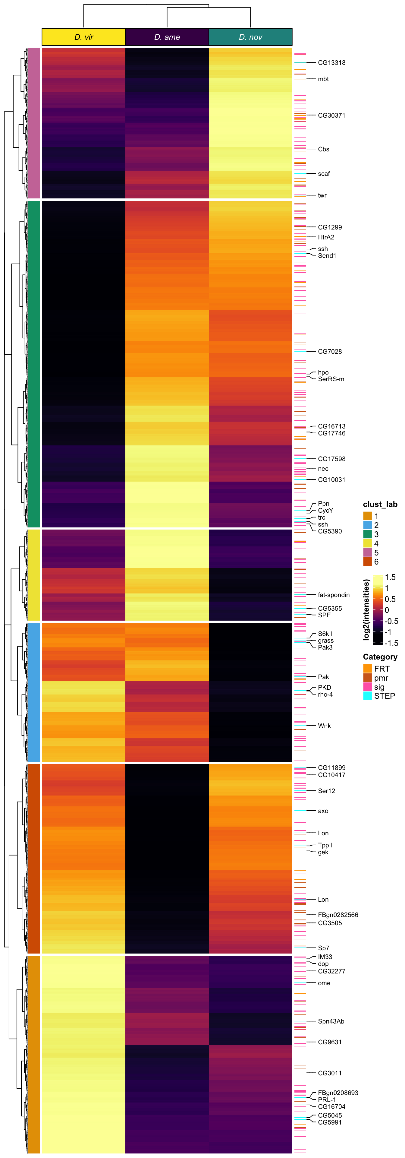
#dev.off()

y2 <- fem_md %>%
  bind_cols(cluster = sub_grpf) %>%
  dplyr::select(genes, FBgn, 9:11, cluster) %>%
  pivot_longer(cols = 3:5) %>%
  mutate(species = str_sub(name, 4, 4))

y2 %>%
  ggplot(aes(x = factor(name, levels = c('D. vir', 'D. ame', 'D. nov')), y = value, fill = name)) +
  geom_boxplot() +
  labs(x = 'Species') +
  scale_fill_viridis_d() +
  facet_wrap(~cluster) +
  ggpubr::stat_compare_means(aes(label = ..p.signif..),
                             comparisons = list(c('D. ame', 'D. nov'),
                                                c('D. ame', 'D. vir'),
                                                c('D. nov', 'D. vir')),
                             method = 't.test') +
  theme_bw() +
  theme(legend.position = '',
        axis.text.x = element_text(face = 'italic')) +
  NULL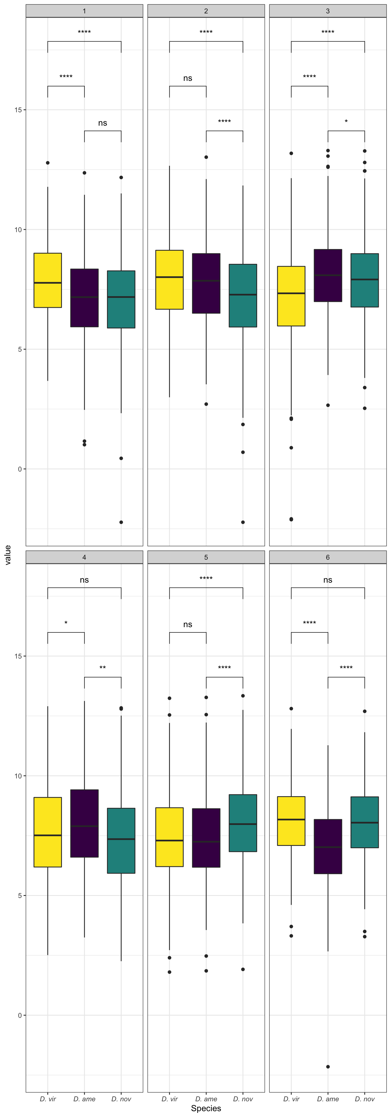
# Model fits
y2 %>% group_by(cluster) %>%
  do(fit = broom::glance(lm(value ~ name, data = .))) %>%
  unnest(fit) %>%
  mutate(p.value = ifelse(p.value < 0.001, '< 0.001', round(p.value, 3))) %>%
  dplyr::select(-adj.r.squared, -sigma, -c(df:df.residual)) %>%
  kable(digits = 3,
        caption = 'Model fits') %>%
kable_styling(full_width = FALSE)| cluster | r.squared | statistic | p.value | nobs |
|---|---|---|---|---|
| 1 | 0.037 | 25.259 | < 0.001 | 1311 |
| 2 | 0.028 | 13.080 | < 0.001 | 921 |
| 3 | 0.041 | 46.667 | < 0.001 | 2163 |
| 4 | 0.017 | 5.127 | 0.006 | 603 |
| 5 | 0.025 | 12.777 | < 0.001 | 999 |
| 6 | 0.103 | 72.134 | < 0.001 | 1254 |
y2 %>% group_by(cluster) %>%
  do(fit = broom::tidy(lm(value ~ name, data = .))) %>%
  unnest(fit) %>%
  mutate(p.value = ifelse(p.value < 0.001, '< 0.001', round(p.value, 3)),
         sigLabel = case_when(p.value < 0.001 ~ "***",
                              p.value < 0.01 ~ "**",
                              p.value < 0.05 ~ "*",
                              TRUE ~ '')) %>%
  kable(digits = 3,
        caption = 'Model estimates') %>%
kable_styling(full_width = FALSE)| cluster | term | estimate | std.error | statistic | p.value | sigLabel |
|---|---|---|---|---|---|---|
| 1 | (Intercept) | 7.140 | 0.082 | 86.734 | < 0.001 | *** |
| 1 | nameD. nov | -0.022 | 0.116 | -0.191 | 0.848 | |
| 1 | nameD. vir | 0.705 | 0.116 | 6.058 | < 0.001 | *** |
| 2 | (Intercept) | 7.809 | 0.105 | 74.345 | < 0.001 | *** |
| 2 | nameD. nov | -0.603 | 0.149 | -4.060 | < 0.001 | *** |
| 2 | nameD. vir | 0.099 | 0.149 | 0.664 | 0.507 | |
| 3 | (Intercept) | 8.068 | 0.065 | 124.689 | < 0.001 | *** |
| 3 | nameD. nov | -0.189 | 0.092 | -2.070 | 0.039 |
|
| 3 | nameD. vir | -0.843 | 0.092 | -9.207 | < 0.001 | *** |
| 4 | (Intercept) | 8.033 | 0.139 | 57.873 | < 0.001 | *** |
| 4 | nameD. nov | -0.617 | 0.196 | -3.143 | 0.002 | ** |
| 4 | nameD. vir | -0.413 | 0.196 | -2.102 | 0.036 |
|
| 5 | (Intercept) | 7.372 | 0.098 | 75.008 | < 0.001 | *** |
| 5 | nameD. nov | 0.612 | 0.139 | 4.399 | < 0.001 | *** |
| 5 | nameD. vir | 0.006 | 0.139 | 0.043 | 0.966 | |
| 6 | (Intercept) | 6.982 | 0.076 | 91.359 | < 0.001 | *** |
| 6 | nameD. nov | 1.088 | 0.108 | 10.070 | < 0.001 | *** |
| 6 | nameD. vir | 1.157 | 0.108 | 10.705 | < 0.001 | *** |
plyr::ldply(lapply(split(y2, y2$cluster, drop = T), function(x)
  {broom::tidy(TukeyHSD(aov(value ~ name, data = x)))})) %>%
  mutate(.id = recode(.id,
                      `D. nov-D. ame` = "D. ame vs. D. nov",
                      `D. vir-D. ame` = "D. ame vs. D. vir",
                      `D. vir-D. nov` = 'D. nov vs. D. vir'),
         across(4:7, ~ round(.x, 2)),
         Estimate = paste0(estimate, ' (', conf.low, '-', conf.high, ')'),
         p.val = ifelse(adj.p.value < 0.001, "< 0.001", round(adj.p.value, 3)),
         sigLabel = case_when(adj.p.value < 0.001 ~ "***",
                              adj.p.value < 0.01 ~ "**",
                              adj.p.value < 0.05 ~ "*",
                              TRUE ~ ''))
.id term contrast null.value estimate conf.low conf.high adj.p.value
1 1 name D. nov-D. ame 0 -0.02 -0.30 0.25 9.800432e-01
2 1 name D. vir-D. ame 0 0.71 0.43 0.98 5.409190e-09
3 1 name D. vir-D. nov 0 0.73 0.45 1.00 1.674723e-09
4 2 name D. nov-D. ame 0 -0.60 -0.95 -0.25 1.575228e-04
5 2 name D. vir-D. ame 0 0.10 -0.25 0.45 7.843046e-01
6 2 name D. vir-D. nov 0 0.70 0.35 1.05 7.979549e-06
7 3 name D. nov-D. ame 0 -0.19 -0.40 0.03 9.626033e-02
8 3 name D. vir-D. ame 0 -0.84 -1.06 -0.63 6.608425e-11
9 3 name D. vir-D. nov 0 -0.65 -0.87 -0.44 6.996403e-11
10 4 name D. nov-D. ame 0 -0.62 -1.08 -0.16 4.987430e-03
11 4 name D. vir-D. ame 0 -0.41 -0.87 0.05 9.026233e-02
12 4 name D. vir-D. nov 0 0.20 -0.26 0.67 5.513659e-01
13 5 name D. nov-D. ame 0 0.61 0.29 0.94 3.577278e-05
14 5 name D. vir-D. ame 0 0.01 -0.32 0.33 9.989762e-01
15 5 name D. vir-D. nov 0 -0.61 -0.93 -0.28 4.340295e-05
16 6 name D. nov-D. ame 0 1.09 0.83 1.34 1.734168e-13
17 6 name D. vir-D. ame 0 1.16 0.90 1.41 1.727507e-13
18 6 name D. vir-D. nov 0 0.07 -0.19 0.32 8.011060e-01
Estimate p.val sigLabel
1 -0.02 (-0.3-0.25) 0.98
2 0.71 (0.43-0.98) < 0.001 ***
3 0.73 (0.45-1) < 0.001 ***
4 -0.6 (-0.95--0.25) < 0.001 ***
5 0.1 (-0.25-0.45) 0.784
6 0.7 (0.35-1.05) < 0.001 ***
7 -0.19 (-0.4-0.03) 0.096
8 -0.84 (-1.06--0.63) < 0.001 ***
9 -0.65 (-0.87--0.44) < 0.001 ***
10 -0.62 (-1.08--0.16) 0.005 **
11 -0.41 (-0.87-0.05) 0.09
12 0.2 (-0.26-0.67) 0.551
13 0.61 (0.29-0.94) < 0.001 ***
14 0.01 (-0.32-0.33) 0.999
15 -0.61 (-0.93--0.28) < 0.001 ***
16 1.09 (0.83-1.34) < 0.001 ***
17 1.16 (0.9-1.41) < 0.001 ***
18 0.07 (-0.19-0.32) 0.801 Differentially abundant proteins only
fem_da <- fem_md %>% filter(genes %in% c(fem_TABLES %>% filter(threshold != 'NS') %>% pull(genes)))

# scale data
mat_scaled_frt2 <- t(apply(fem_da[, 9:11], 1, scale))

# Dissimilarity matrix
df2 <- dist(mat_scaled_frt2, method = "euclidean")

# Hierarchical clustering using Complete Linkage
hc1f2 <- hclust(df2, method = "complete" )

# Plot the dendrogram
#plot(hc1, cex = 0.6, hang = -1)

#fviz_nbclust(mat_scaled_frt2, FUN = hcut, method = "silhouette")

# Cut tree into 4 groups
sub_grpf2 <- cutree(hc1f2, k = 4)

# Number of members in each cluster
#table(sub_grpf2)

cat_labf2 <- rowAnnotation(Cluster = sub_grpf2,
                           col = list(Cluster = setNames(cbPalette[2:5], unique(sub_grpf2))),
                           title = NULL,
                           show_annotation_name = FALSE)

frt_lab <- rowAnnotation(Category = fem_da$fem_cat,
                         col = list(Category = setNames(c('chocolate', 'orange', 'hotpink', 'cyan'),
                                                        na.omit(unique(fem_da$fem_cat)))),
                         frt_labs = anno_mark(at = c(grep('STEP', x = fem_da$fem_cat)),
                                              labels = na.omit(fem_da$Symbol[fem_da$fem_cat == 'STEP']),
                                              labels_gp = gpar(fontsize = 8)),
                         title = NULL,
                         na_col = NA,
                         show_annotation_name = FALSE)

#pdf('plots/frt_compheatmap_da.pdf', height = 8, width = 5)
Heatmap(mat_scaled_frt2,
        col = viridis::inferno(100),
        heatmap_legend_param = list(title = "log2(intensities)",
                                    title_position = "leftcenter-rot"),
        right_annotation = frt_lab,
        left_annotation = cat_labf2,
        top_annotation = haha,
        show_row_names = FALSE,
        show_column_names = FALSE,
        row_split = 4,
        column_split = 3,
        column_gap = unit(0, "mm"),
        row_title = NULL,
        column_title = NULL)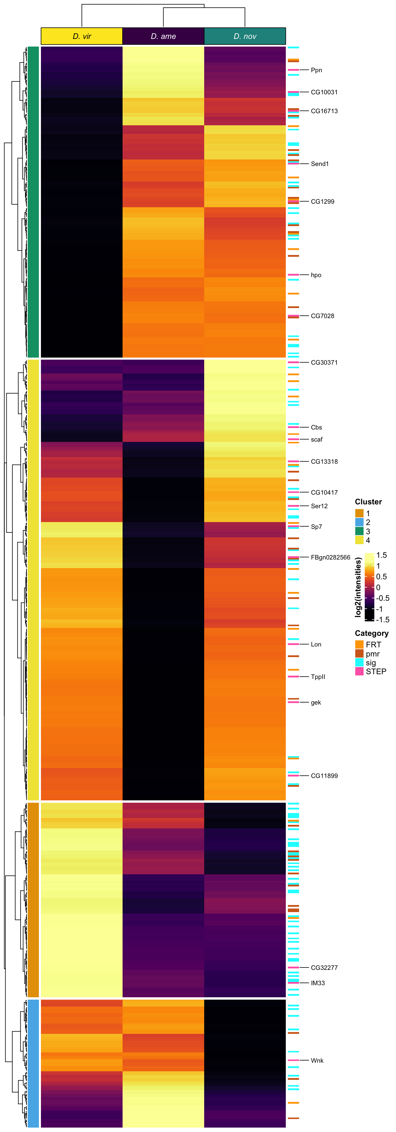
#dev.off()

y3 <- fem_da %>%
  bind_cols(cluster = sub_grpf2) %>%
  dplyr::select(genes, FBgn, 9:11, cluster) %>%
  pivot_longer(cols = 3:5) %>%
  mutate(species = str_sub(name, 4, 4))

y3 %>%
  ggplot(aes(x = factor(name, levels = c('D. vir', 'D. ame', 'D. nov')), y = value, fill = name)) +
  geom_boxplot() +
  labs(x = 'Species') +
  scale_fill_viridis_d() +
  facet_wrap(~cluster) +
  ggsignif::geom_signif(comparisons = list(c("D. ame", "D. nov"),
                                           c("D. ame", "D. vir"),
                                           c("D. nov", "D. vir")),
                        map_signif_level = TRUE) +
  #coord_cartesian(ylim = c(2, 20)) +
  theme_bw() +
  theme(legend.position = '',
        axis.text.x = element_text(face = 'italic')) +
  NULL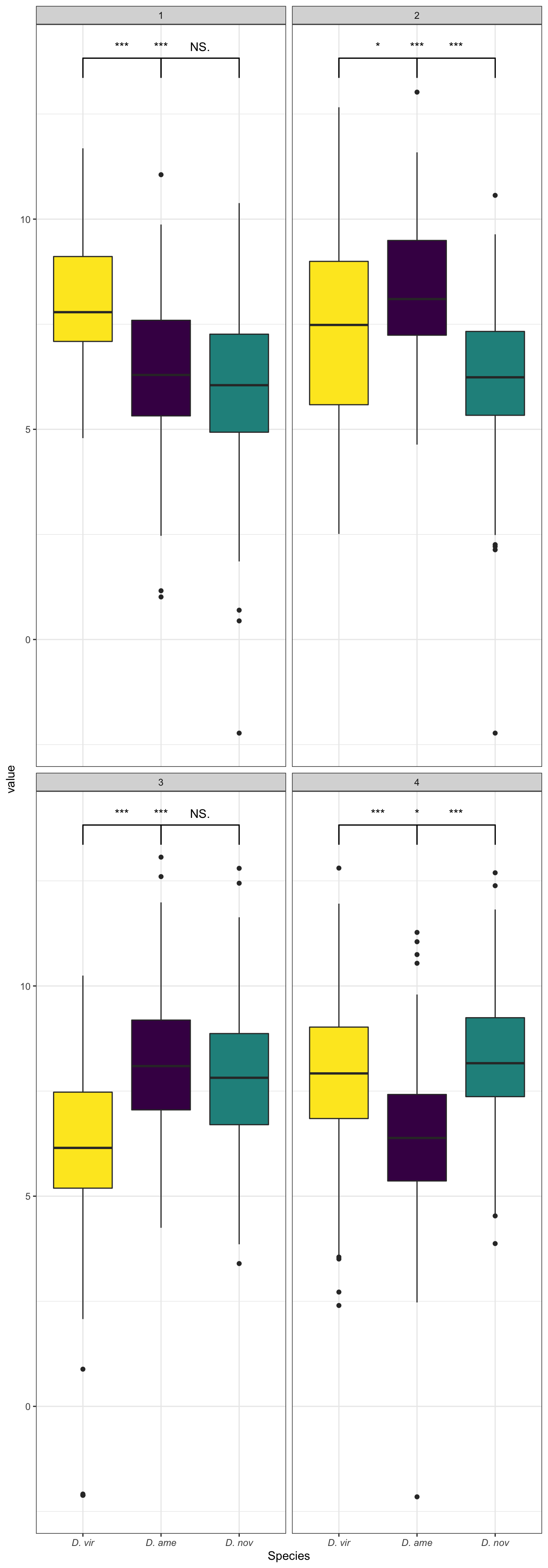
y3 %>%
  mutate(cluster = paste('Cluster', cluster, sep = ' ')) %>%
  ggplot(aes(x = factor(name, levels = c('D. vir', 'D. ame', 'D. nov')), y = value, fill = name)) +
  gghalves::geom_half_point(aes(colour = name)) +
  gghalves::geom_half_violin(aes(fill = name)) +
  stat_pointinterval(pch = 21, fill = 'white') +
  labs(x = 'Species', y = 'normalised abundance') +
  scale_fill_viridis_d() +
  scale_colour_viridis_d() +
  facet_wrap(~cluster, scales = 'free_y') +
  theme_bw() +
  theme(legend.position = '',
        axis.text.x = element_text(face = 'italic')) +
  ggpubr::stat_compare_means(aes(label = ..p.signif..),
                             comparisons = list(c('D. ame', 'D. nov'),
                                                c('D. ame', 'D. vir'),
                                                c('D. nov', 'D. vir')),
                             method = 't.test') +
  #ggsave('plots/frt_pointinterval.pdf', height = 6, width = 6, dpi = 600, useDingbats = FALSE) +
  NULL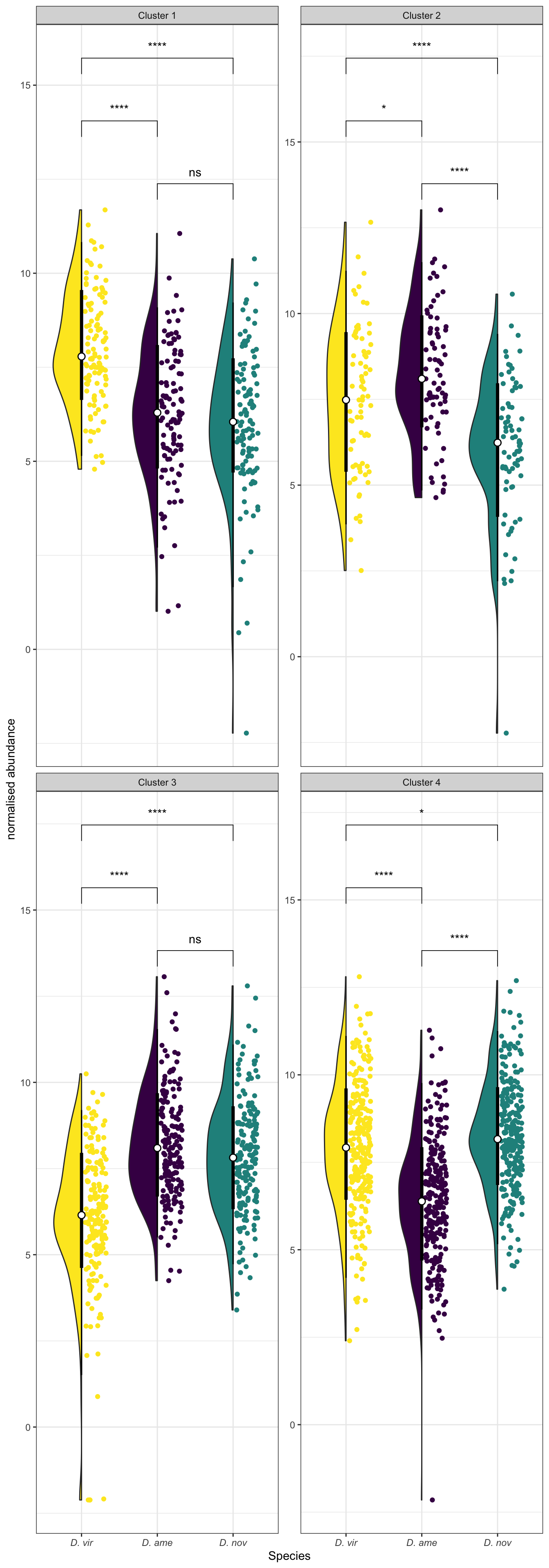
# model fits
y3 %>% group_by(cluster) %>%
  do(fit = broom::tidy(lm(value ~ name, data = .))) %>%
  unnest(fit) %>%
  mutate(p.value = ifelse(p.value < 0.001, '< 0.001', round(p.value, 3)),
         sigLabel = case_when(p.value < 0.001 ~ "***",
                              p.value < 0.01 ~ "**",
                              p.value < 0.05 ~ "*",
                              TRUE ~ '')) %>%
  kable(digits = 3,
        caption = 'Model estimates') %>%
kable_styling(full_width = FALSE)| cluster | term | estimate | std.error | statistic | p.value | sigLabel |
|---|---|---|---|---|---|---|
| 1 | (Intercept) | 6.301 | 0.160 | 39.311 | < 0.001 | *** |
| 1 | nameD. nov | -0.281 | 0.227 | -1.239 | 0.216 | |
| 1 | nameD. vir | 1.711 | 0.227 | 7.548 | < 0.001 | *** |
| 2 | (Intercept) | 8.250 | 0.232 | 35.595 | < 0.001 | *** |
| 2 | nameD. nov | -2.153 | 0.328 | -6.569 | < 0.001 | *** |
| 2 | nameD. vir | -0.781 | 0.328 | -2.382 | 0.018 |
|
| 3 | (Intercept) | 8.178 | 0.132 | 62.113 | < 0.001 | *** |
| 3 | nameD. nov | -0.323 | 0.186 | -1.734 | 0.083 | |
| 3 | nameD. vir | -2.108 | 0.186 | -11.319 | < 0.001 | *** |
| 4 | (Intercept) | 6.399 | 0.105 | 60.722 | < 0.001 | *** |
| 4 | nameD. nov | 1.876 | 0.149 | 12.584 | < 0.001 | *** |
| 4 | nameD. vir | 1.531 | 0.149 | 10.270 | < 0.001 | *** |
# posthoc tests
plyr::ldply(lapply(split(y3, y3$cluster, drop = T), function(x)
  {broom::tidy(TukeyHSD(aov(value ~ name, data = x)))})) %>%
  mutate(.id = recode(.id,
                      `D. nov-D. ame` = "D. ame vs. D. nov",
                      `D. vir-D. ame` = "D. ame vs. D. vir",
                      `D. vir-D. nov` = 'D. nov vs. D. vir'),
         across(4:8, ~ round(.x, 2)),
         Estimate = paste0(estimate, ' (', conf.low, '-', conf.high, ')'),
         sigLabel = case_when(adj.p.value < 0.001 ~ "***",
                              adj.p.value < 0.01 ~ "**",
                              adj.p.value < 0.05 ~ "*",
                              TRUE ~ '')) %>%
  kable(digits = 3,
        caption = 'Post-hoc Tukey tests') %>%
kable_styling(full_width = FALSE)| .id | term | contrast | null.value | estimate | conf.low | conf.high | adj.p.value | Estimate | sigLabel |
|---|---|---|---|---|---|---|---|---|---|
| 1 | name | D. nov-D. ame | 0 | -0.28 | -0.81 | 0.25 | 0.43 | -0.28 (-0.81-0.25) | |
| 1 | name | D. vir-D. ame | 0 | 1.71 | 1.18 | 2.24 | 0.00 | 1.71 (1.18-2.24) | *** |
| 1 | name | D. vir-D. nov | 0 | 1.99 | 1.46 | 2.53 | 0.00 | 1.99 (1.46-2.53) | *** |
| 2 | name | D. nov-D. ame | 0 | -2.15 | -2.93 | -1.38 | 0.00 | -2.15 (-2.93–1.38) | *** |
| 2 | name | D. vir-D. ame | 0 | -0.78 | -1.55 | -0.01 | 0.05 | -0.78 (-1.55–0.01) | |
| 2 | name | D. vir-D. nov | 0 | 1.37 | 0.60 | 2.15 | 0.00 | 1.37 (0.6-2.15) | *** |
| 3 | name | D. nov-D. ame | 0 | -0.32 | -0.76 | 0.11 | 0.19 | -0.32 (-0.76-0.11) | |
| 3 | name | D. vir-D. ame | 0 | -2.11 | -2.55 | -1.67 | 0.00 | -2.11 (-2.55–1.67) | *** |
| 3 | name | D. vir-D. nov | 0 | -1.78 | -2.22 | -1.35 | 0.00 | -1.78 (-2.22–1.35) | *** |
| 4 | name | D. nov-D. ame | 0 | 1.88 | 1.53 | 2.23 | 0.00 | 1.88 (1.53-2.23) | *** |
| 4 | name | D. vir-D. ame | 0 | 1.53 | 1.18 | 1.88 | 0.00 | 1.53 (1.18-1.88) | *** |
| 4 | name | D. vir-D. nov | 0 | -0.34 | -0.69 | 0.01 | 0.05 | -0.34 (-0.69-0.01) |
Evolutionary rates
evo_rates <- kaks_results %>%
  filter(Ka.Ks < 10 & !str_detect(COMPARISON, 'lum')) %>%
  distinct(FBgn, COMPARISON, .keep_all = TRUE) %>%
  mutate(signal_cat = case_when(FBgn %in%
                                  intersect(c(ame_cands$FBgn,
                                              nov_cands$FBgn,
                                              vir_cands$FBgn),
                                            vir_sig$FBgn) ~ 'Ejac.signal',
                                FBgn %in% c(ame_cands$FBgn,
                                               nov_cands$FBgn,
                                               vir_cands$FBgn) ~ 'Ejac',
                                FBgn %in% vir_sig$FBgn ~ 'FRT.signal',
                                FBgn %in% multiDB2$FBgn ~ 'FRT',
                                #FBgn %in% virilisPMDE$FBgn_ID ~ 'pmr',
                                TRUE ~ as.character(NA)),
         STEP = if_else(FBgn %in% STEP$FBgn & signal_cat == 'FRT.signal',
                        'STEP', 'other'))
Signal peptide rates
evo_rates %>%
  drop_na(signal_cat) %>%
  # calculate means and standard errors
  group_by(signal_cat, COMPARISON) %>%
  summarise(mn = mean(Ka.Ks),
            se = sd(Ka.Ks)/sqrt(n())) %>%

  # add mean for all genes
  bind_rows(
    data.frame(kaks_results %>%
                 dplyr::select(COMPARISON, contains('K')) %>%
                 filter(Ka.Ks < 10 & !str_detect(COMPARISON, 'lum'))) %>%
      group_by(COMPARISON) %>%
      summarise(N = n(),
                mn = mean(Ka.Ks),
                se = sd(Ka.Ks)/sqrt(N)) %>%
      mutate(signal_cat = 'All')
            ) %>%

  mutate(cat2 = str_sub(signal_cat, 1, 3),
         cat3 = if_else(grepl('sig', x = signal_cat) == TRUE, 'Signal pep.', 'Other')) %>%

  # plot
  ggplot(aes(x = factor(cat2, level = c('All', 'FRT', 'Eja')),
             y = mn, colour = COMPARISON, shape = cat3)) +
  geom_point(size = 8, position = position_dodge(width = .8)) +
  geom_errorbar(aes(ymin = mn - se, ymax = mn + se), width = .5, position = position_dodge(width = .8)) +
  scale_colour_manual(values = cbPalette[-1],
                      labels = c(D.amr_vs_D.nov = 'D. ame vs. D. nov',
                                 D.amr_vs_D.vir = 'D. ame vs. D. vir',
                                 D.nov_vs_D.vir = 'D. nov vs. D. vir')) +
  scale_x_discrete(labels = c('All', 'Female reproductive\ntract', 'Ejaculate')) +
  scale_shape_manual(values = c(16, 18)) +
  labs(x = 'category', y = 'dN/dS') +
  theme_bw() +
  theme(text = element_text(size = 20),
        legend.position = c(0.25, 0.75),
        legend.title = element_blank(),
        legend.text = element_text(face = "italic"),
        legend.background = element_rect(fill = NA),
        axis.title.x = element_blank()) +
  #ggsave('plots/all_KaKs.pdf', height = 9, width = 8.5, dpi = 600, useDingbats = FALSE) +
  NULL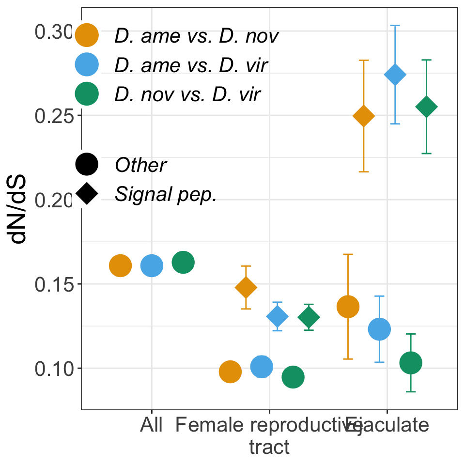
STEP rates
mean_rates <- evo_rates %>%
  group_by(COMPARISON) %>%
  summarise(N = n(),
            mn = mean(Ka.Ks),
            se = sd(Ka.Ks)/sqrt(N)) %>%
  mutate(signal_cat = NA,
         STEP = NA,
         COMPARISON = recode(COMPARISON,
                             D.amr_vs_D.nov = 'D. ame vs. D. nov',
                             D.amr_vs_D.vir = 'D. ame vs. D. vir',
                             D.nov_vs_D.vir = 'D. nov vs. D. vir'))

#plot
evo_rates %>%
  drop_na(signal_cat) %>%
  group_by(signal_cat, STEP, COMPARISON) %>%
  summarise(N = n(),
            mn = mean(Ka.Ks),
            se = sd(Ka.Ks)/sqrt(N)) %>%

  mutate(COMPARISON = recode(COMPARISON,
                             D.amr_vs_D.nov = 'D. ame vs. D. nov',
                             D.amr_vs_D.vir = 'D. ame vs. D. vir',
                             D.nov_vs_D.vir = 'D. nov vs. D. vir')) %>%

  ggplot(aes(x = signal_cat, y = mn, fill = STEP)) +
  geom_hline(data = mean_rates, aes(yintercept = mn), lty = 2, lwd = 1.5) +
  # geom_rect(data = mean_rates, fill = 'black', alpha = .5,
  #           aes(xmin = -Inf, xmax = Inf, ymin = mn - se, ymax = mn + se)) +
  geom_errorbar(aes(ymin = mn - se, ymax = mn + se), position = position_dodge(width = .5),
                width = .5) +
  geom_point(position = position_dodge(width = .5), pch = 21, size = 5) +
  scale_x_discrete(labels = c('Ejac.', 'Ejac.\nsig. pep.',
                              'FRT', 'FRT\nsig. pep.')) +
  scale_fill_manual(values = c('black', 'red')) +
  labs(y = expression(omega)) +
  facet_wrap(~COMPARISON) +
  theme_bw() +
  theme(legend.position = 'bottom',
        legend.title = element_blank(),
        strip.text = element_text(size = 15, face = "italic"),
        axis.title.x = element_blank(),
        axis.title.y = element_text(size = 25),
        axis.text = element_text(size = 15)) +
  geom_text(aes(y = 0.05, label = N), size = 3, position = position_dodge(width = .85)) +
  #ggsave('plots/STEP_KaKs.pdf', height = 4, width = 9.5, dpi = 600, useDingbats = FALSE) +
  NULL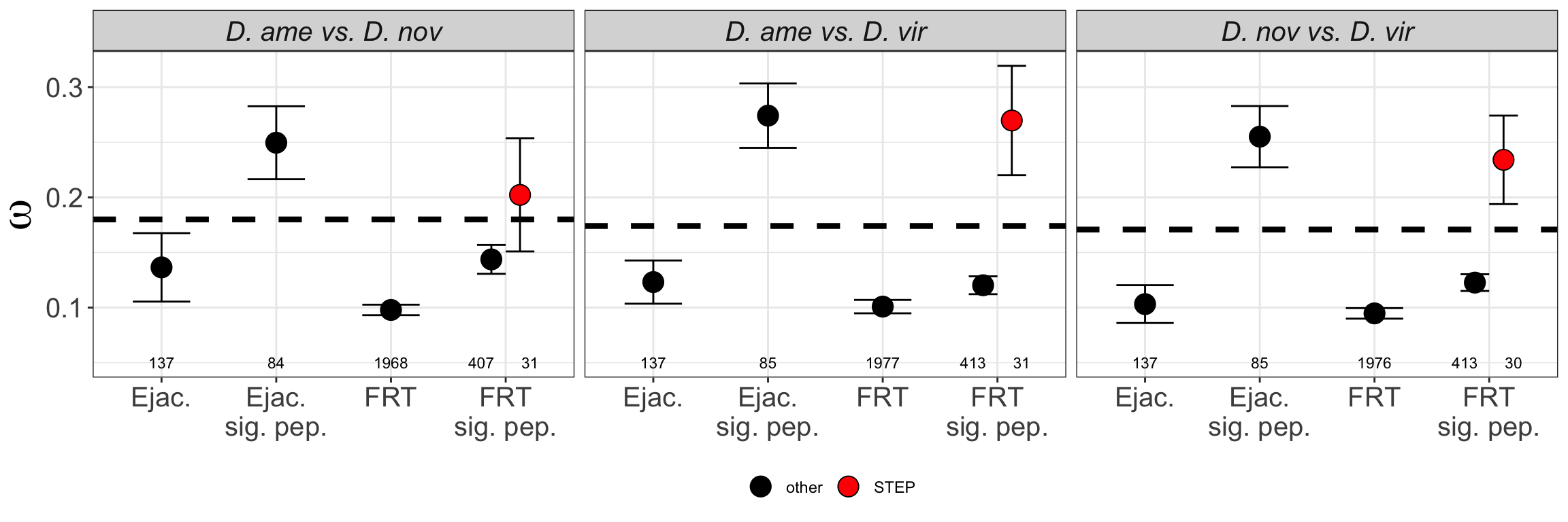
KW tests
bind_rows(

# Ejac (not signal peptides) vs. genome
evo_rates %>%
  mutate(ejac = if_else(grepl('Ejac$', x = signal_cat), 'ejac', 'other')) %>%
  group_by(COMPARISON) %>%
  # ggplot(aes(x = ejac, y = Ka.Ks)) +
  # stat_summary() + facet_wrap(~COMPARISON)
  do(fit = broom::tidy(wilcox.test(Ka.Ks ~ ejac, data = .))) %>%
  unnest(fit),

# ejac.signal vs. genome
evo_rates %>%
  mutate(ejac = if_else(grepl('Ejac.signal', x = signal_cat), 'ejac', 'other')) %>%
  group_by(COMPARISON) %>%
  # ggplot(aes(x = ejac, y = Ka.Ks)) +
  # stat_summary() + facet_wrap(~COMPARISON)
  do(fit = broom::tidy(wilcox.test(Ka.Ks ~ ejac, data = .))) %>%
  unnest(fit),

# ejac.signal vs. ejac.signal + STEP
evo_rates %>%
  filter(str_detect(signal_cat, 'Ejac.signal')) %>%
  dplyr::select(-STEP) %>%
  mutate(STEP = if_else(FBgn %in% STEP$FBgn, 'STEP', 'other')) %>%
  group_by(COMPARISON) %>%
  # ggplot(aes(x = STEP, y = Ka.Ks)) +
  # stat_summary() + facet_wrap(~COMPARISON)
  do(fit = broom::tidy(wilcox.test(Ka.Ks ~ STEP, data = .))) %>%
  unnest(fit),

# ejac/frt w/o signal peptide
evo_rates %>%
  mutate(sex = case_when(grepl('Ejac', x = signal_cat) ~ 'xEjac',
                         grepl('FRT', x = signal_cat) ~ 'xFRT',
                         TRUE ~ as.character(NA)),
         sigp = if_else(grepl('signal', x = signal_cat), 'sigp', 'other')) %>%
  filter(str_detect(sex, 'x')) %>%
  group_by(sex, COMPARISON) %>%
  # ggplot(aes(x = sex, y = Ka.Ks, colour = sigp)) +
  # stat_summary() + facet_wrap(~COMPARISON)
  do(fit = broom::tidy(wilcox.test(Ka.Ks ~ sigp, data = .))) %>%
  unnest(fit),

# frt (not signal peptides) vs. genome
evo_rates %>%
  mutate(frt = if_else(grepl('FRT$', x = signal_cat), 'frt', 'other')) %>%
  group_by(COMPARISON) %>%
  # ggplot(aes(x = frt, y = Ka.Ks)) +
  # stat_summary() + facet_wrap(~COMPARISON)
  do(fit = broom::tidy(wilcox.test(Ka.Ks ~ frt, data = .))) %>%
  unnest(fit),

# FRT.signal vs. genome
evo_rates %>%
  mutate(frt = if_else(grepl('FRT.signal', x = signal_cat), 'frt', 'other')) %>%
  group_by(COMPARISON) %>%
  # ggplot(aes(x = frt, y = Ka.Ks)) +
  # stat_summary() + facet_wrap(~COMPARISON)
  do(fit = broom::tidy(wilcox.test(Ka.Ks ~ frt, data = .))) %>%
  unnest(fit),

# FRT STEP + signal vs. FRT + signal
evo_rates %>%
  filter(str_detect(signal_cat, 'FRT')) %>%
  # ggplot(aes(x = STEP, y = Ka.Ks)) +
  # stat_summary() + facet_wrap(~COMPARISON)
  group_by(COMPARISON) %>%
  do(fit = broom::tidy(wilcox.test(Ka.Ks ~ STEP, data = .))) %>%
  unnest(fit),

# FRT STEP + signal vs. genome
evo_rates %>%
  mutate(STEP = case_when(STEP == 'STEP' ~ 'frt',
                          TRUE ~ 'other')) %>%
  # ggplot(aes(x = STEP, y = Ka.Ks)) +
  # stat_summary() + facet_wrap(~COMPARISON)
  group_by(COMPARISON) %>%
  do(fit = broom::tidy(wilcox.test(Ka.Ks ~ STEP, data = .))) %>%
  unnest(fit),

# FRT STEP vs. Ejac.signal
evo_rates %>%
  mutate(sex = case_when(grepl('Ejac.signal', x = signal_cat) ~ 'Ejac.sig',
                         STEP == 'STEP' ~ 'STEP',
                         TRUE ~ as.character(NA))) %>%
  drop_na(sex) %>%
  group_by(COMPARISON) %>%
  # ggplot(aes(x = sex, y = Ka.Ks)) +
  # stat_summary() + facet_wrap(~COMPARISON)
  do(fit = broom::tidy(wilcox.test(Ka.Ks ~ sex, data = .))) %>%
  unnest(fit)

) %>%
  mutate(pval = ifelse(p.value < 0.001, '< 0.001', round(p.value, 3)),
         sigLabel = case_when(p.value < 0.001 ~ "***",
                              p.value < 0.01 ~ "**",
                              p.value < 0.05 ~ "\\*",
                              TRUE ~ '')) %>%
  dplyr::select(-c(statistic:sex)) %>%
  kable(caption = 'Mann-Whitney U tests comparing evolutionary rates between groups') %>%
  kable_styling(full_width = FALSE) %>%
  group_rows("Ejaculate (excl. sig. peps.) vs. genome", 1, 3) %>%
  group_rows("Ejaculate sig. peps. vs. genome", 4, 6) %>%
  group_rows("Ejaculate sig. peps. vs. Ejaculate sig. peps. + STEP", 7, 9) %>%
  group_rows("Ejaculate with vs. without sig. peps.", 10, 12) %>%
  group_rows("FRT with vs. without sig. peps.", 13, 15) %>%
  group_rows("FRT (excl. sig. peps.) vs. genome", 16, 18) %>%
  group_rows("FRT sig. peps. vs. genome", 19, 21) %>%
  group_rows("FRT STEP w/ sig. peps. vs. FRT w/ sig. peps.", 22, 24) %>%
  group_rows("FRT STEP w/ sig. peps. vs. genome", 25, 27) %>%
group_rows("FRT STEP vs. Ejac.signal", 28, 30)| COMPARISON | pval | sigLabel |
|---|---|---|
| Ejaculate (excl. sig. peps.) vs. genome | ||
| D.amr_vs_D.nov | 0.028 | * |
| D.amr_vs_D.vir | 0.012 | * |
| D.nov_vs_D.vir | < 0.001 | *** |
| Ejaculate sig. peps. vs. genome | ||
| D.amr_vs_D.nov | 0.006 | ** |
| D.amr_vs_D.vir | < 0.001 | *** |
| D.nov_vs_D.vir | < 0.001 | *** |
| Ejaculate sig. peps. vs. Ejaculate sig. peps. + STEP | ||
| D.amr_vs_D.nov | 0.535 | |
| D.amr_vs_D.vir | 0.292 | |
| D.nov_vs_D.vir | 0.424 | |
| Ejaculate with vs. without sig. peps. | ||
| D.amr_vs_D.nov | < 0.001 | *** |
| D.amr_vs_D.vir | < 0.001 | *** |
| D.nov_vs_D.vir | < 0.001 | *** |
| FRT with vs. without sig. peps. | ||
| D.amr_vs_D.nov | < 0.001 | *** |
| D.amr_vs_D.vir | < 0.001 | *** |
| D.nov_vs_D.vir | < 0.001 | *** |
| FRT (excl. sig. peps.) vs. genome | ||
| D.amr_vs_D.nov | < 0.001 | *** |
| D.amr_vs_D.vir | < 0.001 | *** |
| D.nov_vs_D.vir | < 0.001 | *** |
| FRT sig. peps. vs. genome | ||
| D.amr_vs_D.nov | 0.073 | |
| D.amr_vs_D.vir | 0.005 | ** |
| D.nov_vs_D.vir | 0.02 | * |
| FRT STEP w/ sig. peps. vs. FRT w/ sig. peps. | ||
| D.amr_vs_D.nov | 0.002 | ** |
| D.amr_vs_D.vir | < 0.001 | *** |
| D.nov_vs_D.vir | < 0.001 | *** |
| FRT STEP w/ sig. peps. vs. genome | ||
| D.amr_vs_D.nov | 0.489 | |
| D.amr_vs_D.vir | 0.007 | ** |
| D.nov_vs_D.vir | 0.009 | ** |
| FRT STEP vs. Ejac.signal | ||
| D.amr_vs_D.nov | 0.392 | |
| D.amr_vs_D.vir | 0.765 | |
| D.nov_vs_D.vir | 0.916 | |
Database comparisons
Numbers of differentially abundant proteins detected
Here we compare the numbers of differentially abundant proteins detected when using each species databases and the combined database.
Number of ejaculate candidates
Number of proteins more abundant in mated vs. virgin samples
# total number of ejaculate candidates per database
bind_rows(
  ame_DATABLES %>% filter(threshold == 'DA' & str_detect(DA, 'MB')) %>%
    distinct(genes, .keep_all = TRUE),
  nov_DATABLES %>% filter(threshold == 'DA' & str_detect(DA, 'MB')) %>%
    distinct(genes, .keep_all = TRUE),
  vir_DATABLES %>% filter(threshold == 'DA' & str_detect(DA, 'MB')) %>%
    distinct(genes, .keep_all = TRUE),
  comb_TABLES %>% filter(threshold == 'SD' & str_detect(DA, 'MB')) %>%
    distinct(genes, .keep_all = TRUE) %>%
    mutate(threshold = recode(threshold, SD = "DA"), DB = 'aa.comb') %>%
    dplyr::select(species, DB, threshold)) %>%
  group_by(DB) %>%
  dplyr::count() %>%
  left_join(data.frame(DB = c('aa.comb', 'ame.db', 'nov.db', 'vir.db'),
                       total = c(n_distinct(comb_TABLES$genes),
                                 n_distinct(ame_DATABLES$genes),
                                 n_distinct(nov_DATABLES$genes),
                                 n_distinct(vir_DATABLES$genes)))) %>%
  mutate(prop.ejac = n/total)
# A tibble: 4 × 4
# Groups: DB [4]
DB n total prop.ejac
<chr> <int> <int> <dbl>
1 aa.comb 206 2645 0.0779
2 ame.db 346 4020 0.0861
3 nov.db 322 3899 0.0826
4 vir.db 264 3785 0.0697ejac_counts <- bind_rows(
ame_DATABLES %>% filter(threshold == 'DA' & str_detect(DA, 'MB')),
nov_DATABLES %>% filter(threshold == 'DA' & str_detect(DA, 'MB')),
vir_DATABLES %>% filter(threshold == 'DA' & str_detect(DA, 'MB')),
comb_TABLES %>% filter(threshold == 'SD' & str_detect(DA, 'MB')) %>%
mutate(threshold = recode(threshold, SD = "DA"), DB = 'aa.comb') %>%
dplyr::select(species, DB, threshold)) %>%
group_by(species, DB) %>%
dplyr::count()
ejac_counts %>%
ggplot(aes(x = species, y = n, fill = DB)) +
geom_col(position = 'dodge') +
scale_x_discrete(labels = c(expression(italic('D. ame')),
expression(italic('D. nov')),
expression(italic('D. vir')))) +
scale_fill_manual(values = c(viridis::magma(n = 4)[3], viridis::viridis(n = 3)),
name = "Database:",
labels = c('Combined',
expression(italic('D. ame')),
expression(italic('D. nov')),
expression(italic('D. vir')))) +
labs(y = 'No. proteins') +
theme_bw() +
theme(legend.position = 'bottom',
legend.background = element_rect(fill = NA),
axis.title.x = element_blank()) +
#ggsave('plots/database_comps/n_ejac_comb.pdf', height = 3, width = 4, dpi = 600, useDingbats = FALSE) +
NULL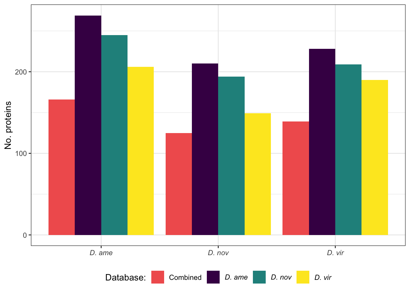
Differentially abundant ejaculate candidates
Number of proteins detected as differentially abundant in pairwise comparisons between species
ejac_da <- bind_rows(ame_MATED %>% filter(threshold == 'DA') %>%
                       dplyr::select(comparison, DB, threshold),
                     nov_MATED %>% filter(threshold == 'DA') %>%
                       dplyr::select(comparison, DB, threshold),
                     vir_MATED %>% filter(threshold == 'DA') %>%
                       dplyr::select(comparison, DB, threshold),
                     mated_TABLES %>% filter(threshold == 'SD') %>%
                       mutate(comparison = recode(comparison,
                                                  aMn = "ame.v.nov",
                                                  aMv = "ame.v.vir",
                                                  nMv = 'nov.v.vir'),
                              threshold = recode(threshold, SD = "DA"),
                              DB = 'aa.comb') %>%
                       dplyr::select(comparison, DB, threshold))

# number of DA ejaculate proteins for each species by database
ejac_da %>%
  group_by(comparison, DB) %>% dplyr::count() %>%
  ggplot(aes(x = comparison, y = n, fill = DB)) +
  geom_col(position = 'dodge') +
  scale_x_discrete(labels = c(expression(italic('D. ame vs. D. nov')),
                              expression(italic('D. ame vs. D. vir')),
                              expression(italic('D. nov vs. D. vir')))) +
  scale_fill_manual(values = c(viridis::magma(n = 4)[3], viridis::viridis(n = 3)),
                    name = "Database:",
                    labels = c('Combined',
                               expression(italic('D. ame')),
                               expression(italic('D. nov')),
                               expression(italic('D. vir')))) +
  labs(y = 'No. proteins') +
  theme_bw() +
  theme(legend.position = 'bottom',
        legend.background = element_rect(fill = NA),
        axis.title.x = element_blank()) +
  #ggsave('plots/database_comps/n_DA_comb.pdf', height = 3, width = 4, dpi = 600, useDingbats = FALSE) +
  NULL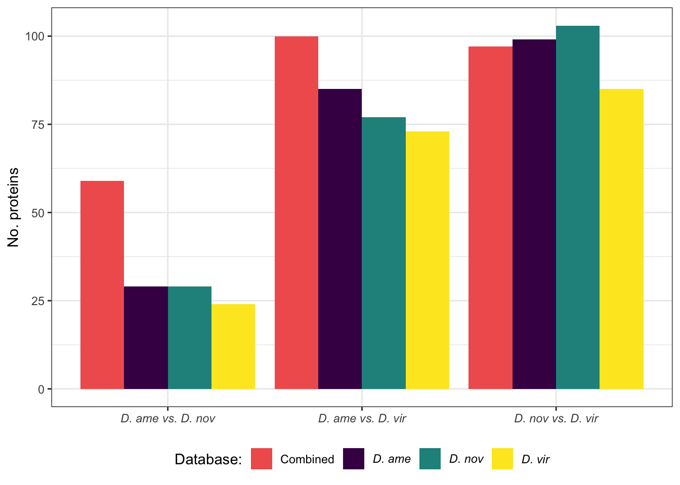
Differentially abundant female reproductive tract proteins
Number of proteins detected as differentially abundant in pairwise comparisons between species
frt_da <- bind_rows(ame_VIRGIN %>% filter(threshold == 'DA') %>%
                      dplyr::select(comparison, DB, threshold),
                    nov_VIRGIN %>% filter(threshold == 'DA') %>%
                      dplyr::select(comparison, DB, threshold),
                    vir_VIRGIN %>% filter(threshold == 'DA') %>%
                      dplyr::select(comparison, DB, threshold),
                    fem_TABLES %>% filter(threshold == 'SD') %>%
                      mutate(comparison = recode(comparison,
                                                 aVn = "ame.v.nov",
                                                 aVv = "ame.v.vir",
                                                 nVv = 'nov.v.vir'),
                             threshold = recode(threshold, SD = "DA"),
                             DB = 'aa.comb') %>%
                      dplyr::select(comparison, DB, threshold))

frt_da %>%
  group_by(comparison, DB) %>% dplyr::count() %>%
  ggplot(aes(x = comparison, y = n, fill = DB)) +
  geom_col(position = 'dodge') +
  scale_x_discrete(labels = c(expression(italic('D. ame vs. D. nov')),
                              expression(italic('D. ame vs. D. vir')),
                              expression(italic('D. nov vs. D. vir')))) +
  scale_fill_manual(values = c(viridis::magma(n = 4)[3], viridis::viridis(n = 3)),
                    name = "Database:",
                    labels = c('Combined',
                               expression(italic('D. ame')),
                               expression(italic('D. nov')),
                               expression(italic('D. vir')))) +
  labs(y = 'No. proteins') +
  theme_bw() +
  theme(legend.position = 'bottom',
        legend.background = element_rect(fill = NA),
        axis.title.x = element_blank()) +
  #ggsave('plots/database_comps/n_DAfem_comb.pdf', height = 3, width = 4, dpi = 600, useDingbats = FALSE) +
  NULL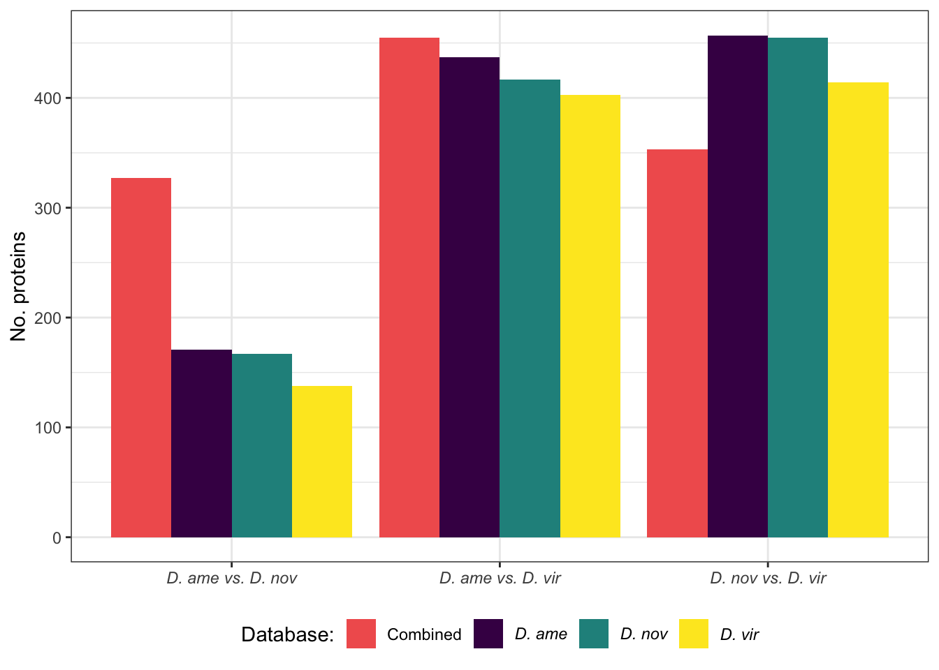
Proportions detected
bind_rows(ejac_counts %>%
            left_join(data.frame(DB = c('aa.comb', 'ame.db', 'nov.db', 'vir.db'),
                                 total = c(n_distinct(comb_TABLES$genes),
                                           n_distinct(ame_DATABLES$genes),
                                           n_distinct(nov_DATABLES$genes),
                                           n_distinct(vir_DATABLES$genes)))) %>%
            mutate(set = 'Ejaculate candidates',
                   comparison = species),
          ejac_da %>%
            group_by(comparison, DB) %>% dplyr::count() %>%
            left_join(data.frame(DB = c('aa.comb', 'ame.db', 'nov.db', 'vir.db'),
                                 total = c(n_distinct(mated_TABLES$genes),
                                           n_distinct(ame_MATED$genes),
                                           n_distinct(nov_MATED$genes),
                                           n_distinct(vir_MATED$genes)))) %>%
            mutate(set = 'Ejaculate divergence'),
          frt_da %>%
            group_by(comparison, DB) %>% dplyr::count() %>%
            left_join(data.frame(DB = c('aa.comb', 'ame.db', 'nov.db', 'vir.db'),
                                 total = c(n_distinct(fem_TABLES$genes),
                                           n_distinct(ame_VIRGIN$genes),
                                           n_distinct(nov_VIRGIN$genes),
                                           n_distinct(vir_VIRGIN$genes)))) %>%
            mutate(set = 'FRT divergence')) %>%
  mutate(prop.da = n/total) %>%
  ggplot(aes(x = comparison, y = prop.da, colour = DB)) +
  geom_line(aes(group = DB), lwd = 2) +
  scale_x_discrete(labels = c(expression(italic('D. ame vs. D. nov')),
                              expression(italic('D. ame vs. D. vir')),
                              expression(italic('D. nov vs. D. vir')))) +
  scale_y_continuous(labels = scales::percent) +
  scale_colour_manual(values = c(viridis::magma(n = 4)[3], viridis::viridis(n = 3)),
                    name = "Database",
                    labels = c('Combined',
                               expression(italic('D. ame')),
                               expression(italic('D. nov')),
                               expression(italic('D. vir')))) +
  labs(y = '% differentially abundant') +
  facet_wrap(~set, scales = 'free', nrow = 1) +
  theme_bw() +
  theme(#legend.position = 'bottom',
        legend.text.align = 0,
        legend.background = element_rect(fill = NA),
        axis.title.x = element_blank(),
        axis.text.x = element_text(size = 8),
        strip.text = element_text(size = 15)) +
  #ggsave('plots/database_comps/prop_DA.pdf', height = 3.8, width = 13.5, dpi = 600, useDingbats = FALSE) +
  NULL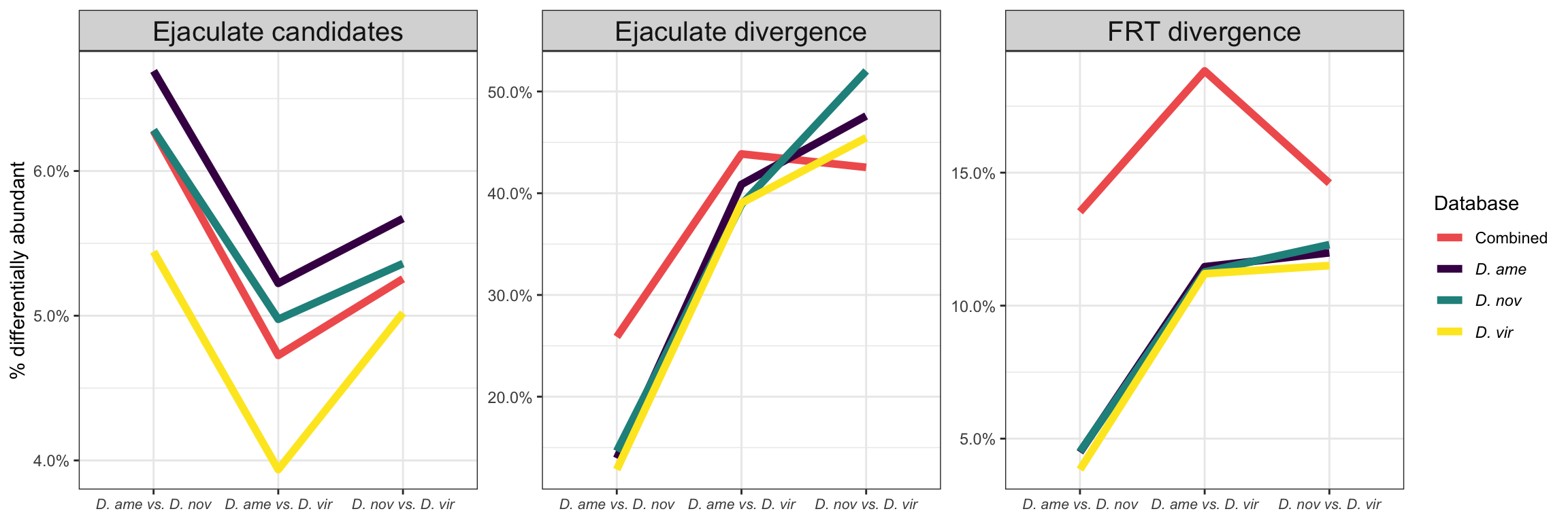
Compare summary statistics
bind_rows(recip_dat %>%
            select(starts_with('Coverage.in.Percent')) %>% cor %>% reshape2::melt(),
          recip_dat %>% select(starts_with('Number.of.PSMs')) %>% log10 %>% cor %>% reshape2::melt(),
          recip_dat %>% select(starts_with('Number.of.Unique.Peptides')) %>% cor %>% reshape2::melt(),
          recip_dat %>% select(starts_with('Number.of.AAs')) %>% log10 %>% cor %>% reshape2::melt(),
          recip_dat %>% select(starts_with('MW.in.kDa')) %>% log10 %>% cor %>% reshape2::melt(),
          recip_dat %>% select(starts_with('calc.pI')) %>% cor %>% reshape2::melt(),
          recip_dat %>% select(starts_with('Score.Mascot.Mascot')) %>% cor %>% reshape2::melt(),
          recip_dat %>% select(starts_with('Number.of.Peptides.by.Search.Engine.Mascot')) %>% log10 %>% cor %>%
            reshape2::melt()) %>%
  filter(Var1 != Var2) %>%
  distinct(value, .keep_all = TRUE) %>%
  mutate(var = gsub('_.*', '', Var1),
         comp = paste(str_sub(Var2, -3), str_sub(Var1, -3), sep = '_'),
         var = gsub('Number.of.Peptides.by.Search.Engine.Mascot', 'N.peptides.by.Mascot', x = var)) %>%
  ggplot(aes(x = var, y = value, colour = comp)) +
  geom_point(size = 5) +
  labs(y = 'Pearson\'s correlation') +
  scale_colour_manual(values = cbPalette[-1],
                      labels = c(expression(paste(italic('D. ame'), ' vs. ', italic('D. ame'))),
                                 expression(paste(italic('D. ame'), ' vs. ', italic('D. vir'))),
                                 expression(paste(italic('D. nov'), ' vs. ', italic('D. vir'))))) +
  theme_bw() +
  theme(legend.position = 'bottom',
        legend.title = element_blank(),
        axis.text.x = element_text(angle = 45, hjust = 1),
        axis.title.x = element_blank()) +
  #ggsave('plots/database_comps/summary_correlations.pdf', height = 4, width = 3, dpi = 600, useDingbats = FALSE) +
  NULL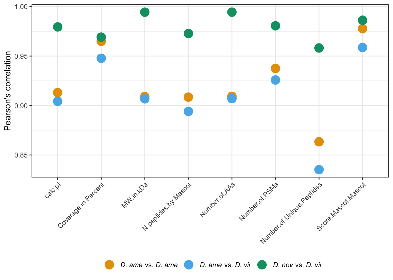
Abundance correlations
Here we compare the protein abundances when searching against each species proteome. We will use sample AM as a test set of data. First, we average the abundances for each search by taking the mean across all three replicates of AM (1-3).
all_abund <- recip_dat %>%
  select(Accession_vir, FBgn,
         starts_with('AV'), starts_with('AM'),
         starts_with('NV'), starts_with('NM'),
         starts_with('VV'), starts_with('VM')) %>%
  mutate(across(3:50, ~replace_na(.x, 0)))

abund_cor <- bind_rows(
  # correlations between replicates within treatment using species specific DB
  all_abund %>% dplyr::select(-Accession_vir, -FBgn) %>% +1 %>% log2 %>% cor() %>%
  reshape2::melt() %>%
  mutate(condition1 = str_sub(Var1, 1, 2),
         condition2 = str_sub(Var2, 1, 2),
         sample1 = str_sub(Var1, 1, 3),
         sample2 = str_sub(Var2, 1, 3),
         db1 = str_sub(Var1, 5, 7),
         db2 = str_sub(Var2, 5, 7)) %>%
  filter(condition1 == condition2) %>%
  filter(Var1 != Var2) %>%
  filter(db1 == db2) %>%
  distinct(value, .keep_all = TRUE) %>%

  # calculate means and standard errors
  group_by(condition1, db1, db2) %>%
  summarise(N = n(),
            mn = mean(value),
            se = sd(value)/sqrt(N)) %>%
  filter(str_sub(tolower(condition1), 1, 1) == str_sub(db1, 1, 1)),

  # correlations between replicates using alt. species DB
  all_abund %>% dplyr::select(-Accession_vir, -FBgn) %>% +1 %>% log2 %>% cor() %>%
  reshape2::melt() %>%
  mutate(condition1 = str_sub(Var1, 1, 2),
         condition2 = str_sub(Var2, 1, 2),
         sample1 = str_sub(Var1, 1, 3),
         sample2 = str_sub(Var2, 1, 3),
         db1 = str_sub(Var1, 5, 7),
         db2 = str_sub(Var2, 5, 7)) %>%
  filter(sample1 == sample2) %>%
  filter(db1 != db2) %>%
  distinct(Var1, Var2, .keep_all = TRUE) %>%

  # calculate means and standard errors
  group_by(condition1, db1, db2) %>%
  summarise(N = n(),
            mn = mean(value),
            se = sd(value)/sqrt(N)) %>%
  filter(str_sub(tolower(condition1), 1, 1) == str_sub(db1, 1, 1))
  )

abund_cor$NAMEX <- c('AMA', 'AVA', 'NMN', 'NVN', 'VMV', 'VVV',
                     'AMN', 'AMV', 'AVN', 'AVV', 'NMA', 'NMV',
                     'NVA', 'NVV', 'VMA', 'VMN', 'VVA', 'VVN')

# plot
abund_cor %>%
  ggplot(aes(x = condition1, y = mn, colour = db2)) +
  geom_errorbar(aes(ymin = mn - se, ymax = mn + se), width = .5) +
  geom_point(size = 5)  +
  labs(y = 'Pearson\'s correlation') +
  scale_colour_viridis_d(name = "Database:",
                         labels = c(expression(italic('D. ame')),
                                    expression(italic('D. nov')),
                                    expression(italic('D. vir')))) +
  theme_bw() +
  theme(legend.position = 'bottom',
        legend.text.align = 0,
        axis.title.x = element_blank()) +
  #ggsave('plots/database_comps/abun_correlations.pdf', height = 4.25, width = 4, dpi = 600, useDingbats = FALSE) +
  NULL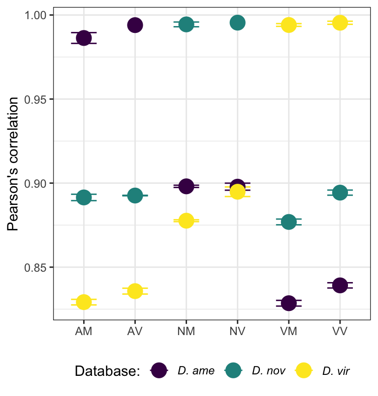
Coefficients of variation
We calculate the coefficient of variation for each treatment (mated or virgin within each species); (1) between biological replicates within each treatment using each species database as a measure of precision and (2) between each sample using each database as a measure of variation between databases.
# function to calculate CV
cv <- function(x) sd(x, na.rm = TRUE)/mean(x, na.rm = TRUE)

# combine data across individual databases
all_vals <- bind_rows(ame_Dat %>%
                        dplyr::select(Accession, AM1:VV3) %>%
                        rename_with(.cols = 2:17, function(x) {paste0('ame.', x)}) %>%
                        pivot_longer(2:17),
                      nov_Dat %>%
                        dplyr::select(Accession, AM1:VV3) %>%
                        rename_with(.cols = 2:17, function(x) {paste0('nov.', x)}) %>%
                        pivot_longer(2:17),
                      vir_Dat %>%
                        dplyr::select(Accession, AM1:VV3) %>%
                        rename_with(.cols = 2:17, function(x) {paste0('vir.', x)}) %>%
                        pivot_longer(2:17)) %>%
  mutate(log_val = log10(value + 1),
         db = str_sub(name, 1, 3),
         condition = str_sub(name, 5, 6),
         .sample = str_sub(name, 5, 7))

# CV for entire experiment using each database
all_vals %>%
  group_by(Accession, db) %>%
  summarise(CV = cv(log_val)) %>%
  group_by(db) %>%
  summarise(N = n(),
            md = median(CV, na.rm = TRUE),
            mn = mean(CV, na.rm = TRUE),
            se = sd(CV, na.rm = TRUE)/sqrt(N)) %>%
  ggplot(aes(x = db, y = mn, fill = db)) +
  geom_errorbar(aes(ymin = mn - se, ymax = mn + se), width = 0) +
  geom_point(pch = 21, size = 5) +
  scale_fill_viridis_d() +
  scale_x_discrete(labels = c('ame' = expression(italic('D. ame')),
                              'nov' = expression(italic('D. nov')),
                              'vir' = expression(italic('D. vir')))) +
  labs(x = 'Database', y = 'CV') +
  theme_bw() +
  theme(legend.position = '') +
  NULL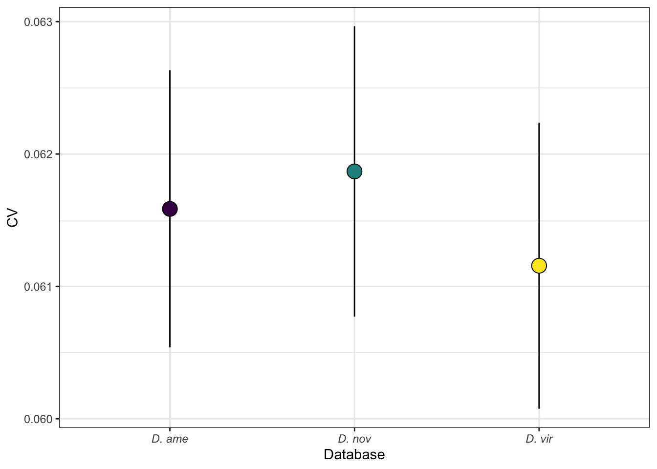
# compare CVs within each condition using each database
all_vals %>%
  group_by(Accession, db, condition) %>%
  summarise(CV = cv(log_val)) %>%
  group_by(db, condition) %>%
  summarise(N = n(),
            md = median(CV, na.rm = TRUE),
            mn = mean(CV, na.rm = TRUE),
            se = sd(CV, na.rm = TRUE)/sqrt(N)) %>%
  ggplot(aes(x = condition, y = mn, fill = db)) +
  geom_errorbar(aes(ymin = mn - se, ymax = mn + se), width = 0,
                position = position_dodge(width = .5)) +
  geom_point(pch = 21, position = position_dodge(width = .5)) +
  scale_fill_viridis_d(name = "Database:",
                       labels = c('ame' = expression(italic('D. ame')),
                                  'nov' = expression(italic('D. nov')),
                                  'vir' = expression(italic('D. vir')))) +
  labs(y = 'CV') +
  theme_bw() +
  theme(legend.position = 'bottom') +
  #ggsave('plots/database_comps/CV_within_treatment_db.pdf', height = 8, width = 12, units = 'cm', dpi = 600, useDingbats = FALSE) +
  NULL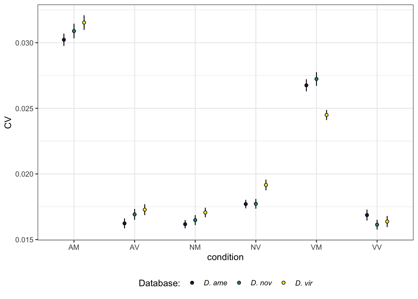
| Version | Author | Date |
|---|---|---|
| f28e7a0 | MartinGarlovsky | 2022-02-07 |
# compare samples across different databases using the combined database to allow comparison between the same proteins across databases.
all_abund %>%
  pivot_longer(3:50) %>%
  mutate(log_val = log10(value),
         db = str_sub(name, 5, 7),
         condition = str_sub(name, 1, 2),
         .sample = str_sub(name, 1, 3)) %>%
  group_by(FBgn, .sample) %>%
  summarise(CV = cv(log_val)) %>%
  group_by(.sample) %>%
  summarise(N = n(),
            md = median(CV, na.rm = TRUE),
            mn = mean(CV, na.rm = TRUE),
            se = sd(CV, na.rm = TRUE)/sqrt(N)) %>%
  ggplot(aes(x = .sample, y = mn)) +
  geom_errorbar(aes(ymin = mn - se, ymax = mn + se), width = 0) +
  geom_point(size = 5) +
  labs(y = 'CV') +
  theme_bw() +
  theme(legend.position = 'bottom') +
  #ggsave('plots/database_comps/CV_btw_sample_db.pdf', height = 5, width = 15, units = 'cm', dpi = 600, useDingbats = FALSE) +
  NULL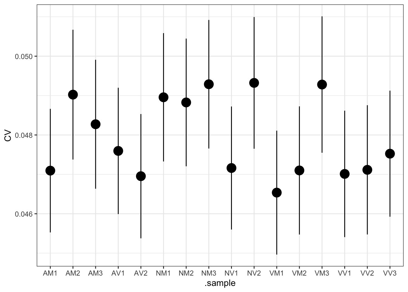
| Version | Author | Date |
|---|---|---|
| f28e7a0 | MartinGarlovsky | 2022-02-07 |
Test differences in abundances between databases
We compared differences in abundance between databases for each species/mating combination using edgeR. Significant differences in abundance indicate that using each species data provides different estimates of protein abundance.
Heatmap
abun_mn <- all_abund %>%
  mutate(mn = rowMeans(dplyr::select(., -c(1:2)), na.rm = TRUE)) %>%
  filter(mn > 0) %>%
  mutate(AMA = rowMeans(dplyr::select(., matches("AM._ame")), na.rm = TRUE),
         AVA = rowMeans(dplyr::select(., matches("AV._ame")), na.rm = TRUE),
         AMN = rowMeans(dplyr::select(., matches("AM._nov")), na.rm = TRUE),
         AVN = rowMeans(dplyr::select(., matches("AV._nov")), na.rm = TRUE),
         AMV = rowMeans(dplyr::select(., matches("AM._vir")), na.rm = TRUE),
         AVV = rowMeans(dplyr::select(., matches("AV._vir")), na.rm = TRUE),

         NMA = rowMeans(dplyr::select(., matches("NM._ame")), na.rm = TRUE),
         NVA = rowMeans(dplyr::select(., matches("NV._ame")), na.rm = TRUE),
         NMN = rowMeans(dplyr::select(., matches("NM._nov")), na.rm = TRUE),
         NVN = rowMeans(dplyr::select(., matches("NV._nov")), na.rm = TRUE),
         NMV = rowMeans(dplyr::select(., matches("NM._vir")), na.rm = TRUE),
         NVV = rowMeans(dplyr::select(., matches("NV._vir")), na.rm = TRUE),

         VMA = rowMeans(dplyr::select(., matches("VM._ame")), na.rm = TRUE),
         VVA = rowMeans(dplyr::select(., matches("VV._ame")), na.rm = TRUE),
         VMN = rowMeans(dplyr::select(., matches("VM._nov")), na.rm = TRUE),
         VVN = rowMeans(dplyr::select(., matches("VV._nov")), na.rm = TRUE),
         VMV = rowMeans(dplyr::select(., matches("VM._vir")), na.rm = TRUE),
         VVV = rowMeans(dplyr::select(., matches("VV._vir")), na.rm = TRUE)) %>%
  dplyr::select(!contains('_'), -mn)

# scale data
scaled_comp <- t(apply(log2(abun_mn[, -1] + 1), 1, scale))

colnames(scaled_comp) <- colnames(abun_mn[, -1])

sp_anno <- str_sub(colnames(abun_mn[, -1]), 1, 1)
mt_anno <- str_sub(colnames(abun_mn[, -1]), 2, 2)
db_anno <- str_sub(colnames(abun_mn[, -1]), 3, 3)

# get column names for ordering
v <- colnames(scaled_comp)

ha <- HeatmapAnnotation(
  species = str_sub(colnames(abun_mn[, -1]), 1, 1),
  mating = str_sub(colnames(abun_mn[, -1]), 2, 2),
  database = str_sub(colnames(abun_mn[, -1]), 3, 3),
  col = list(species = c('V' = v.pal[1],
                         'N' = v.pal[2],
                         'A' = v.pal[3]),
             mating = c('M' = viridis::magma(n = 4)[3],
                        'V' = viridis::magma(n = 4)[2]),
             database = c('V' = v.pal[1],
                          'N' = v.pal[2],
                          'A' = v.pal[3])
             )
  # cors = anno_points(
  #   abund_cor[match(v[order(substr(v, start = 1,
  #                                  stop = max(nchar(v))))], abund_cor$NAMEX), 'mn'])
  )

#pdf('plots/database_comps/db_comp_compheatmap.pdf', height = 8, width = 5)
Heatmap(scaled_comp,
        col = RColorBrewer::brewer.pal(name = 'Spectral', n = 15),
        heatmap_legend_param = list(title = "log2(intensities)",
                                    title_position = "leftcenter-rot"),
        column_order = v[order(substr(v, start = 1, stop = max(nchar(v))))],
        #right_annotation = frt_labs,
        #left_annotation = frt_lab,
        top_annotation = ha,
        show_row_names = FALSE,
        show_column_names = FALSE,
        column_gap = unit(0, "mm"),
        row_title = NULL,
        column_title = NULL)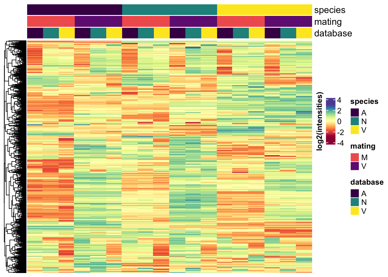
#dev.off()Density plots
data.frame(FBgn = abun_mn$FBgn,
           scaled_comp) %>%
  pivot_longer(cols = 2:19) %>%
  separate(name, into = c('condition', 'database'), sep = 2, remove = FALSE) %>%
  ggplot(aes(x = value, y = database, fill = database)) +
  ggridges::geom_density_ridges() +
  scale_fill_viridis_d() +
  labs(x = 'log2(scaled abundance)', y = 'Database') +
  facet_wrap(~condition, ncol = 2) +
  theme_bw() +
  theme(legend.position = '')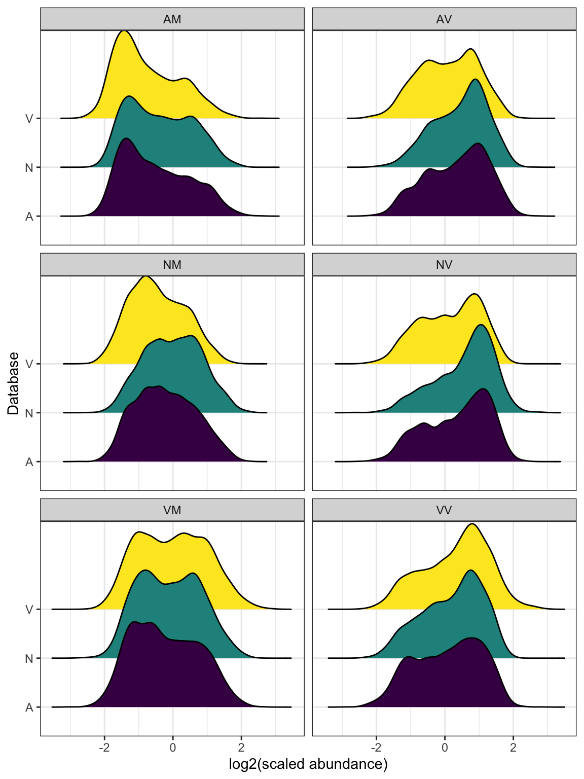
Differential abundance analysis
# subset data for each condition using all databases
am_dat <- all_abund %>% dplyr::select(Accession_vir, FBgn, starts_with('AM'))
av_dat <- all_abund %>% dplyr::select(Accession_vir, FBgn, starts_with('AV'))

nm_dat <- all_abund %>% dplyr::select(Accession_vir, FBgn, starts_with('NM'))
nv_dat <- all_abund %>% dplyr::select(Accession_vir, FBgn, starts_with('NV'))

vm_dat <- all_abund %>% dplyr::select(Accession_vir, FBgn, starts_with('VM'))
vv_dat <- all_abund %>% dplyr::select(Accession_vir, FBgn, starts_with('VV'))

# function to perform differential abundance analysis between databases for the
# same samples

do_limma <- function(df) {

  expr_dat = df[, -c(1:2)]

  # get sample info
  sampInfo = data.frame(database = str_sub(colnames(expr_dat), 5, 7),
                        Replicate = str_sub(colnames(expr_dat), 3, 3))

  # make design matrix to test diffs between groups
  design = model.matrix(~0 + sampInfo$database)
  colnames(design) = unique(sampInfo$database)
  rownames(design) = sampInfo$Replicate

  # create DGElist and fit model
  dgeList = DGEList(counts = expr_dat, genes = df$Accession_vir, group = sampInfo$database)
  dgeList = calcNormFactors(dgeList, method = 'TMM')
  dgeList = estimateCommonDisp(dgeList)
  dgeList = estimateTagwiseDisp(dgeList)

  # make contrasts - higher values = higher alphabetically
  cont.matrix = makeContrasts(a.vs.n = ame - nov,
                              a.vs.v = ame - vir,
                              n.vs.v = nov - vir,
                              levels = design)

  # voom normalisation
  dgeListV = voom(dgeList, design, plot = FALSE)

  # fit linear model
  lm_fit <- lmFit(dgeListV, design = design)

  # compare differential abundance between databases
  # ame vs. nov
  lm_an = contrasts.fit(lm_fit, cont.matrix[,"a.vs.n"])
  lm_an = eBayes(lm_an)
  lm_an.tTags.table = topTable(lm_an, adjust.method = "BH", number = Inf) %>%
    mutate(comparison = "a.vs.n",
           threshold = if_else(adj.P.Val < 0.05 & abs(logFC) > 1, "SD", "NS"))

  # ame vs. vir
  lm_av <- contrasts.fit(lm_fit, cont.matrix[,"a.vs.v"])
  lm_av <- eBayes(lm_av)
  lm_av.tTags.table <- topTable(lm_av, adjust.method = "BH", number = Inf) %>%
    mutate(comparison = "a.vs.v",
           threshold = if_else(adj.P.Val < 0.05 & abs(logFC) > 1, "SD", "NS"))

  # nov vs. vir
  lm_nv <- contrasts.fit(lm_fit, cont.matrix[,"n.vs.v"])
  lm_nv <- eBayes(lm_nv)
  lm_nv.tTags.table <- topTable(lm_nv, adjust.method = "BH", number = Inf) %>%
    mutate(comparison = "n.vs.v",
           threshold = if_else(adj.P.Val < 0.05 & abs(logFC) > 1, "SD", "NS"))

  # combine results
  return(rbind(lm_an.tTags.table, lm_av.tTags.table, lm_nv.tTags.table))

}


combi_2 <- bind_rows(do_limma(am_dat) %>% mutate(dat = 'AM'),
                     do_limma(av_dat) %>% mutate(dat = 'AV'),
                     do_limma(nm_dat) %>% mutate(dat = 'NM'),
                     do_limma(nv_dat) %>% mutate(dat = 'NV'),
                     do_limma(vm_dat) %>% mutate(dat = 'VM'),
                     do_limma(vv_dat) %>% mutate(dat = 'VV')) %>%
  left_join(vir_ids, by = c('genes' = 'prot_id')) %>%
  mutate(comparison = recode(comparison,
                             a.vs.n = "D.amr_vs_D.nov",
                             a.vs.v = "D.amr_vs_D.vir",
                             n.vs.v = 'D.nov_vs_D.vir')) %>%
  # add evolutionary rates
  left_join(kaks_results %>% dplyr::select(Ka:COMPARISON, FBgn),
            by = c('FBgn', c('comparison' = 'COMPARISON'))) %>%
  distinct(FBgn, comparison, dat, .keep_all = TRUE)

# volcanos
combi_2 %>%
  ggplot(aes(x = logFC, y = -log10(P.Value), colour = threshold)) +
  geom_point(alpha = .5) +
  labs(y = '-log10(p-value)') +
  facet_grid(dat~comparison) +
  theme_bw() +
  theme(legend.position = '') +
  NULL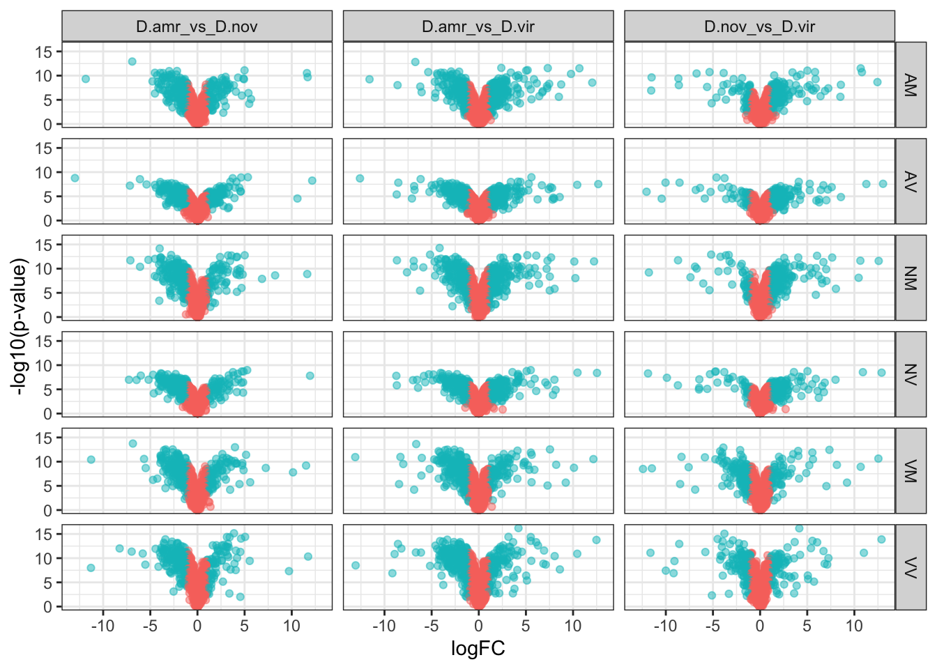
# # numbers differentially abundant
# combi_2 %>%
#   group_by(dat, comparison) %>%
#   count(threshold) %>%
#   ggplot(aes(x = comparison, y = n, fill = threshold)) +
#   geom_col() +
#   facet_wrap(~dat)
#
# # percent different in estimate
# combi_2 %>%
#   group_by(dat, comparison) %>%
#   count(threshold) %>%
#   group_by(dat, comparison) %>%
#   summarise(p.diff = 100 * n[threshold == 'SD']/(n[threshold == 'SD'] + n[threshold == 'NS'])) %>%
#   summary
Evolutionary rates
We compare dN/dS for proteins that showed differences in abundance when using each species database. We expect faster evolving proteins will be more likely differentially abundant between databases if amino acid substitutions lead to less accurate peptide assignment/abundance estimates.
combi_2 %>% filter(Ka.Ks < 10) %>%
  mutate(condition = str_sub(dat, 2, 2)) %>%
  group_by(comparison, threshold, condition) %>%
  summarise(N = n(),
            mn = mean(Ka.Ks),
            se = sd(Ka.Ks)/sqrt(N)) %>%
  ggplot(aes(x = comparison, y = mn, fill = threshold, shape = condition)) +
  geom_errorbar(aes(ymin = mn - se, ymax = mn + se), width = 0,
                position = position_dodge(width = .5)) +
  geom_point(size = 3, position = position_dodge(width = .5)) +
  labs(x = 'Database comparison', y = expression(omega)) +
  scale_shape_manual(values = c(21:22),
                     labels = c('M' = 'Mated',
                                'V' = 'Virgin')) +
  scale_fill_manual(values = cbPalette[-1]) +
  scale_x_discrete(labels =
                     c('D.amr_vs_D.nov' =
                         expression(paste(italic('D. ame'), ' vs. ', italic('D. nov'))),
                       'D.amr_vs_D.vir' =
                         expression(paste(italic('D. ame'), ' vs. ', italic('D. vir'))),
                       'D.nov_vs_D.vir' =
                         expression(paste(italic('D. nov'), ' vs. ', italic('D. vir'))))) +
  guides(fill = guide_legend(override.aes = list(shape = 21))) +
  theme_bw() +
  theme(#legend.position = 'bottom',
        legend.title = element_blank(),
        axis.text.x = element_text(angle = 15, hjust = 1),
        axis.title.y = element_text(size = 25)) +
  #ggsave('plots/database_comps/db_comp_rates.pdf', height = 9, width = 11, units = 'cm', dpi = 600, useDingbats = FALSE) +
  NULL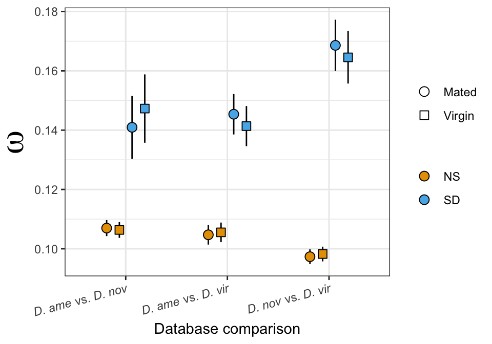
# perform KW tests
kw_rates <- combi_2 %>% filter(Ka.Ks < 10) %>%
  group_by(dat, comparison) %>%
  do(fit = broom::tidy(wilcox.test(Ka.Ks ~ threshold, data = .))) %>%
  unnest(fit)

kw_rates$FDR <- p.adjust(kw_rates$p.value, method = 'fdr')

kw_rates %>%
  mutate(FDR = ifelse(FDR < 0.001, '< 0.001', round(FDR, 3)),
         sigLabel = case_when(FDR < 0.001 ~ "***",
                              FDR < 0.01 ~ "**",
                              FDR < 0.05 ~ "\\*",
                              TRUE ~ '')) %>%
  dplyr::select(-c(p.value:alternative)) %>%
  kable(digits = 3,
        caption = 'Wilcoxon rank sum test with continuity correction') %>%
kable_styling(full_width = FALSE)| dat | comparison | statistic | FDR | sigLabel |
|---|---|---|---|---|
| AM | D.amr_vs_D.nov | 297172.0 | 0.007 | ** |
| AM | D.amr_vs_D.vir | 351296.5 | < 0.001 | *** |
| AM | D.nov_vs_D.vir | 202603.0 | < 0.001 | *** |
| AV | D.amr_vs_D.nov | 279638.5 | 0.002 | ** |
| AV | D.amr_vs_D.vir | 351005.5 | < 0.001 | *** |
| AV | D.nov_vs_D.vir | 196326.5 | < 0.001 | *** |
| NM | D.amr_vs_D.nov | 298230.0 | 0.002 | ** |
| NM | D.amr_vs_D.vir | 364372.0 | < 0.001 | *** |
| NM | D.nov_vs_D.vir | 209933.0 | < 0.001 | *** |
| NV | D.amr_vs_D.nov | 283477.5 | < 0.001 | *** |
| NV | D.amr_vs_D.vir | 358542.5 | < 0.001 | *** |
| NV | D.nov_vs_D.vir | 188287.5 | < 0.001 | *** |
| VM | D.amr_vs_D.nov | 297534.0 | 0.006 | ** |
| VM | D.amr_vs_D.vir | 359691.0 | < 0.001 | *** |
| VM | D.nov_vs_D.vir | 209270.5 | < 0.001 | *** |
| VV | D.amr_vs_D.nov | 291328.5 | 0.024 | * |
| VV | D.amr_vs_D.vir | 370468.0 | < 0.001 | *** |
| VV | D.nov_vs_D.vir | 208473.5 | < 0.001 | *** |
Similarly, we expect proteins without orthologs to be less abundant.
all_dat <- bind_rows(
  ame_abund %>%
    left_join(recip_dat %>% dplyr::select(Accession_ame, Orthogroup),
              by = c('Accession' = 'Accession_ame')) %>%
    mutate(AM = rowMeans(select(., starts_with('AM')), na.rm = TRUE),
           AV = rowMeans(select(., starts_with('AV')), na.rm = TRUE),
           NM = rowMeans(select(., starts_with('NM')), na.rm = TRUE),
           NV = rowMeans(select(., starts_with('NV')), na.rm = TRUE),
           VM = rowMeans(select(., starts_with('VM')), na.rm = TRUE),
           VV = rowMeans(select(., starts_with('VV')), na.rm = TRUE),
           ave_abundance = rowMeans(select(., AM1:VV3), na.rm = TRUE)) %>%
    mutate(DB = 'ame'),
  nov_abund %>%
    left_join(recip_dat %>% dplyr::select(Accession_nov, Orthogroup),
              by = c('Accession' = 'Accession_nov')) %>%
    mutate(AM = rowMeans(select(., starts_with('AM')), na.rm = TRUE),
           AV = rowMeans(select(., starts_with('AV')), na.rm = TRUE),
           NM = rowMeans(select(., starts_with('NM')), na.rm = TRUE),
           NV = rowMeans(select(., starts_with('NV')), na.rm = TRUE),
           VM = rowMeans(select(., starts_with('VM')), na.rm = TRUE),
           VV = rowMeans(select(., starts_with('VV')), na.rm = TRUE),
           ave_abundance = rowMeans(select(., AM1:VV3), na.rm = TRUE)) %>%
    mutate(DB = 'nov'),
  vir_abund %>%
    left_join(recip_dat %>% dplyr::select(Accession_vir, Orthogroup),
              by = c('Accession' = 'Accession_vir')) %>%
    mutate(AM = rowMeans(select(., starts_with('AM')), na.rm = TRUE),
           AV = rowMeans(select(., starts_with('AV')), na.rm = TRUE),
           NM = rowMeans(select(., starts_with('NM')), na.rm = TRUE),
           NV = rowMeans(select(., starts_with('NV')), na.rm = TRUE),
           VM = rowMeans(select(., starts_with('VM')), na.rm = TRUE),
           VV = rowMeans(select(., starts_with('VV')), na.rm = TRUE),
           ave_abundance = rowMeans(select(., AM1:VV3), na.rm = TRUE)) %>%
    mutate(DB = 'vir')) %>%
  mutate(ortholog = if_else(is.na(Orthogroup), 'no', 'yes'))

# # check average expression is similar between edgeR/manual calculation
# ame_MATED %>%
#   left_join(all_dat, by = c('genes' = 'Accession')) %>%
#   drop_na(ave_abundance) %>%
#   ggplot(aes(x = AveExpr, y = log2(ave_abundance), colour = ortholog)) +
#   geom_point()

all_dat %>%
  ggplot(aes(x = DB, y = log2(ave_abundance), fill = ortholog)) +
  #stat_summary(position = position_dodge(width = .5), size = 2, pch = 21) +
  geom_boxplot(notch = TRUE) +
  labs(x = 'Database', y = 'log2(abundance)') +
  scale_x_discrete(labels = c('ame' = expression(italic('D. ame')),
                              'nov' = expression(italic('D. nov')),
                              'vir' = expression(italic('D. vir')))) +
  theme_bw() +
  theme(legend.position = 'bottom') +
  #ggsave('plots/database_comps/orth_abun.pdf', height = 9, width = 8.8, units = 'cm', dpi = 600, useDingbats = FALSE) +
  NULL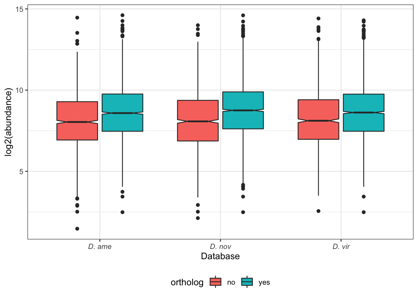
# perform KW tests
all_dat %>%
  group_by(DB) %>%
  do(fit = broom::tidy(wilcox.test(ave_abundance ~ ortholog, data = .))) %>%
  unnest(fit) %>%
  mutate(p.value = ifelse(p.value < 0.001, '< 0.001', round(p.value, 3)),
         sigLabel = case_when(p.value < 0.001 ~ "***",
                              p.value < 0.01 ~ "**",
                              p.value < 0.05 ~ "*",
                              TRUE ~ '')) %>%
  dplyr::select(-c(method:alternative)) %>%
  kable(digits = 3,
        caption = 'Wilcoxon rank sum test with continuity correction') %>%
kable_styling(full_width = FALSE)| DB | statistic | p.value | sigLabel |
|---|---|---|---|
| ame | 1509198 | < 0.001 | *** |
| nov | 1333776 | < 0.001 | *** |
| vir | 1295576 | < 0.001 | *** |
sessionInfo()R version 4.0.3 (2020-10-10)
Platform: x86_64-apple-darwin17.0 (64-bit)
Running under: macOS Big Sur 10.16
Matrix products: default
BLAS: /Library/Frameworks/R.framework/Versions/4.0/Resources/lib/libRblas.dylib
LAPACK: /Library/Frameworks/R.framework/Versions/4.0/Resources/lib/libRlapack.dylib
locale:
[1] en_GB.UTF-8/en_GB.UTF-8/en_GB.UTF-8/C/en_GB.UTF-8/en_GB.UTF-8
attached base packages:
[1] grid stats graphics grDevices utils datasets methods
[8] base
other attached packages:
[1] factoextra_1.0.7 cluster_2.1.2 ape_5.5
[4] DT_0.18 kableExtra_1.3.4 edgeR_3.32.1
[7] limma_3.46.0 eulerr_6.1.0 RColorBrewer_1.1-2
[10] UpSetR_1.4.0 ComplexHeatmap_2.9.3 ggrepel_0.9.1
[13] tidybayes_3.0.1 forcats_0.5.1 stringr_1.4.0
[16] dplyr_1.0.7 purrr_0.3.4 readr_2.0.1
[19] tidyr_1.1.4 tibble_3.1.5 ggplot2_3.3.5
[22] tidyverse_1.3.1 workflowr_1.6.2
loaded via a namespace (and not attached):
[1] readxl_1.3.1 backports_1.2.1 circlize_0.4.13
[4] systemfonts_1.0.2 plyr_1.8.6 splines_4.0.3
[7] polylabelr_0.2.0 svUnit_1.0.6 digest_0.6.28
[10] foreach_1.5.1 htmltools_0.5.1.1 viridis_0.6.1
[13] fansi_0.5.0 magrittr_2.0.1 checkmate_2.0.0
[16] doParallel_1.0.16 openxlsx_4.2.4 tzdb_0.1.2
[19] modelr_0.1.8 matrixStats_0.60.0 vroom_1.5.4
[22] svglite_2.0.0 colorspace_2.0-2 rvest_1.0.1
[25] ggdist_3.0.0 haven_2.4.3 xfun_0.25
[28] crayon_1.4.2 jsonlite_1.7.2 iterators_1.0.13
[31] glue_1.5.0 polyclip_1.10-0 gtable_0.3.0
[34] webshot_0.5.2 GetoptLong_1.0.5 distributional_0.2.2
[37] car_3.0-11 shape_1.4.6 BiocGenerics_0.36.1
[40] abind_1.4-5 scales_1.1.1 DBI_1.1.1
[43] rstatix_0.7.0 Rcpp_1.0.7 viridisLite_0.4.0
[46] clue_0.3-59 foreign_0.8-81 bit_4.0.4
[49] stats4_4.0.3 htmlwidgets_1.5.3 httr_1.4.2
[52] arrayhelpers_1.1-0 posterior_1.0.1 ellipsis_0.3.2
[55] pkgconfig_2.0.3 farver_2.1.0 sass_0.4.0
[58] dbplyr_2.1.1 locfit_1.5-9.4 utf8_1.2.2
[61] tidyselect_1.1.1 labeling_0.4.2 rlang_0.4.12
[64] reshape2_1.4.4 later_1.3.0 munsell_0.5.0
[67] cellranger_1.1.0 tools_4.0.3 cli_3.1.0
[70] generics_0.1.1 ggridges_0.5.3 broom_0.7.9
[73] evaluate_0.14 yaml_2.2.1 knitr_1.33
[76] bit64_4.0.5 fs_1.5.0 zip_2.2.0
[79] nlme_3.1-152 whisker_0.4 xml2_1.3.2
[82] compiler_4.0.3 rstudioapi_0.13 curl_4.3.2
[85] png_0.1-7 ggsignif_0.6.2 reprex_2.0.1
[88] bslib_0.2.5.1 stringi_1.7.5 highr_0.9
[91] lattice_0.20-44 Matrix_1.3-4 tensorA_0.36.2
[94] vctrs_0.3.8 pillar_1.6.4 lifecycle_1.0.1
[97] jquerylib_0.1.4 GlobalOptions_0.1.2 data.table_1.14.0
[100] httpuv_1.6.2 R6_2.5.1 promises_1.2.0.1
[103] rio_0.5.27 gridExtra_2.3 IRanges_2.24.1
[106] codetools_0.2-18 assertthat_0.2.1 rprojroot_2.0.2
[109] rjson_0.2.20 withr_2.4.2 S4Vectors_0.28.1
[112] mgcv_1.8-36 parallel_4.0.3 hms_1.1.0
[115] gghalves_0.1.1 coda_0.19-4 rmarkdown_2.10
[118] carData_3.0-4 Cairo_1.5-12.2 ggpubr_0.4.0
[121] git2r_0.28.0 lubridate_1.7.10