TPP-analysis
MartinGarlovsky
2022-10-25
Last updated: 2022-12-01
Checks: 7 0
Knit directory: virilisProteomics/
This reproducible R Markdown analysis was created with workflowr (version 1.7.0). The Checks tab describes the reproducibility checks that were applied when the results were created. The Past versions tab lists the development history.
Great! Since the R Markdown file has been committed to the Git repository, you know the exact version of the code that produced these results.
Great job! The global environment was empty. Objects defined in the global environment can affect the analysis in your R Markdown file in unknown ways. For reproduciblity it’s best to always run the code in an empty environment.
The command set.seed(20201210) was run prior to running
the code in the R Markdown file. Setting a seed ensures that any results
that rely on randomness, e.g. subsampling or permutations, are
reproducible.
Great job! Recording the operating system, R version, and package versions is critical for reproducibility.
Nice! There were no cached chunks for this analysis, so you can be confident that you successfully produced the results during this run.
Great job! Using relative paths to the files within your workflowr project makes it easier to run your code on other machines.
Great! You are using Git for version control. Tracking code development and connecting the code version to the results is critical for reproducibility.
The results in this page were generated with repository version f18ceb3. See the Past versions tab to see a history of the changes made to the R Markdown and HTML files.
Note that you need to be careful to ensure that all relevant files for
the analysis have been committed to Git prior to generating the results
(you can use wflow_publish or
wflow_git_commit). workflowr only checks the R Markdown
file, but you know if there are other scripts or data files that it
depends on. Below is the status of the Git repository when the results
were generated:
Ignored files:
    Ignored:    .DS_Store
    Ignored:    .RData
    Ignored:    .Rhistory
    Ignored:    .Rproj.user/
    Ignored:    analysis/.DS_Store
    Ignored:    analysis/.Rhistory
    Ignored:    code/.DS_Store
    Ignored:    data/.DS_Store
    Ignored:    output/.DS_Store

Untracked files:
    Untracked:  .Rapp.history
    Untracked:  TrialDataFirstLook.R
    Untracked:  alignment_dotplot_dark_AN.png
    Untracked:  code/.ipynb_checkpoints/
    Untracked:  code/find_seq.py
    Untracked:  comparisons/
    Untracked:  data/ABetal.2020/
    Untracked:  data/Big_table_virilis_group_with_divergence_geneflow_Leeban.csv
    Untracked:  data/Dvir_stringtie_transcripts_lengths.txt
    Untracked:  data/FlyBase_GO_STEP.txt
    Untracked:  data/Garlovsky_etal_Dmon_MaxQuant_ParkerID.csv
    Untracked:  data/Orthogroups.tsv
    Untracked:  data/PEAKS/
    Untracked:  data/ProteomeDiscoverer/
    Untracked:  data/RNASeq_data/
    Untracked:  data/SPN_ids.csv
    Untracked:  data/mRNA_abundances/
    Untracked:  data/melanogaster/
    Untracked:  data/orthology_matching/
    Untracked:  data/reciprocal_orths.csv
    Untracked:  data/signal_peptides/
    Untracked:  data/vir_annotation.rds
    Untracked:  data/virilis_Accession2FBgn_uniprot.csv
    Untracked:  data/virilis_male_AG_SFP_EB_genes.txt
    Untracked:  data/virilis_molecular_evolution_results/
    Untracked:  output/ClueGOlists/
    Untracked:  output/all_ejac_IDs.csv
    Untracked:  output/combined_database.csv
    Untracked:  output/combined_database_tpp.csv
    Untracked:  output/duplicated_proteins.csv
    Untracked:  output/ejac_IDs_no-orths.csv
    Untracked:  plots/

Unstaged changes:
    Deleted:    analysis/data-exploration.Rmd
    Deleted:    analysis/differential-abundance.Rmd
    Modified:   analysis/multi-database.Rmd
    Modified:   code/mRNA_integration_analysis.ipynb
Note that any generated files, e.g. HTML, png, CSS, etc., are not included in this status report because it is ok for generated content to have uncommitted changes.
These are the previous versions of the repository in which changes were
made to the R Markdown (analysis/TPP-analysis.Rmd) and HTML
(docs/TPP-analysis.html) files. If you’ve configured a
remote Git repository (see ?wflow_git_remote), click on the
hyperlinks in the table below to view the files as they were in that
past version.
| File | Version | Author | Date | Message |
|---|---|---|---|---|
| Rmd | f18ceb3 | MartinGarlovsky | 2022-12-01 | wflow_publish("analysis/TPP-analysis.Rmd") |
Introduction
The following analyses are the results of a 16-plex TMT labelling proteomics experiment. Flies were flash frozen in liquid nitrogen within ~30 seconds after copulation ended and stored at -80ºC. Later, female flies were thawed and the lower reproductive tract dissected with fine forceps in a drop of 1X PBS, rinsed in a second drop, and then added to a pool (n = ) of XXX kept on ice. Samples were shipped on dry ice to the Cambridge Core Proteomics Facility, UK, for LC-MS/MS. Resulting .raw files were processed in Proteome Discoverer using each species’ proteome.
Load packages
library(tidyverse)
library(tidybayes)
library(ggrepel)
library(ComplexHeatmap)
library(ggalluvial)
library(cluster)
library(factoextra)
library(grid)
library(UpSetR)
library(RColorBrewer)
library(eulerr)
library(edgeR)
library(kableExtra)
#library(DT)

# colour palettes

# colourblind friendly palette
cbPalette <- c("#999999", "#E69F00", "#56B4E9", "#009E73", "#F0E442", "#CC79A7", "#D55E00", "#0072B2", "#CC79A7")

# viridis palettes
v.pal <- viridis::viridis(n = 3, direction = -1)
m.pal <- viridis::magma(n = 5, direction = -1)
c.pal <- viridis::inferno(n = 7)

# met brewer egypt palette
egypt.pal <- MetBrewer::met.brewer('Egypt')

# nice tables
my_data_table <- function(df){
  datatable(
    df, rownames = FALSE,
    autoHideNavigation = TRUE,
    extensions = c("Scroller",  "Buttons"),
    options = list(
      dom = 'Bfrtip',
      deferRender = TRUE,
      scrollX = TRUE, scrollY = 400,
      scrollCollapse = TRUE,
      buttons =
        list('csv', list(
          extend = 'pdf',
          pageSize = 'A4',
          orientation = 'landscape',
          filename = 'Dpseudo_respiration')),
      pageLength = 50
    )
  )
}
Load data
Peptide abundance data exported from TransProteomicPipeline using each species search
Trinotate gene annotations for D. virilis and .gff
virilis group accessory gland, ejaculatory bulb and seminal fluid protein genes
List of D. melanogaster sperm protein orthologs from Wasborough et al. (2009), comprising 1108 proteins, combined with the DmSP1
List of putative D. melanogaster Sfps identified by Wigby et al. (2020). Phil. trans. B
Orthology table between D. melanogaster and D. virilis FBgns
Male accessory gland or ejaculatory bulb biased genes and putative SFPs from Ahmed-Braimah et al. (2017) G3
Female reproductive tract biased genes and postmating response genes from Ahmed-Braimah et al. (2021) MBE
Pairwise dN/dS results also from Ahmed-Braimah et al. (2021) MBE
Signal peptide predictions for each species from SignalP-5.0
Gene ontology (GO) information for all D. virilis genes from FlyBase.org
Orthofinder orthogroups results for reciprocal orthology between species for all proteins
Load peptide intensities and calculate protein abudnances
We load results from the TPP and filter peptides and proteins before calculating protein abundance across all peptides for a given protein.
# correct column names for intensities
new.names <- c('AM1', 'AM2', 'AM3', 'AV1', 'AV2', 'NM1', 'NM2', 'NM3', 'NV1', 'NV2', 'VM1', 'VM2', 'VM3', 'VV1', 'VV2', 'VV3')

# load TPP data and give proper names to abundance columns, filter out decoy peptides and those without sufficient evidence
tmt_ame <- read.delim('../TPP_aalysis/DameSB_db/OUTPUT/combined/TMT_quant.tsv',
                      na.strings = "") %>% rename(protein = X.protein) %>%
  drop_na(peptide) %>%
  filter(!str_detect(protein, 'DECOY'), kept. == 'Yes') %>%
  select(protein, peptide, contains("inten"))
colnames(tmt_ame)[3:18] <- new.names

tmt_nov <- read.delim('../TPP_aalysis/Dnov14_db/OUTPUT/combined/TMT_quant.tsv',
                      na.strings = "") %>% rename(protein = X.protein) %>%
  drop_na(peptide) %>%
  filter(!str_detect(protein, 'DECOY'), kept. == 'Yes') %>%
  select(protein, peptide, contains("inten"))
colnames(tmt_nov)[3:18] <- new.names

tmt_vir <- read.delim('../TPP_aalysis/Dvir87_db/OUTPUT/combined/TMT_quant.tsv',
                      na.strings = "") %>% rename(protein = X.protein) %>%
  drop_na(peptide) %>%
  filter(!str_detect(protein, 'DECOY'), kept. == 'Yes') %>%
  select(protein, peptide, contains("inten"))
colnames(tmt_vir)[3:18] <- new.names

# # extract peptide stats
# tmt_ame_stats <- read.delim('../TPP_aalysis/DameSB_db/OUTPUT/combined/TMT_quant.tsv',
#                       na.strings = "") %>%
#   distinct(protein, .keep_all = TRUE) %>%
#   select(protein, protratio0:proterr15)
#
# tmt_nov_stats <- read.delim('../TPP_aalysis/Dnov14_db/OUTPUT/combined/TMT_quant.tsv',
#                       na.strings = "") %>%
#   distinct(protein, .keep_all = TRUE) %>%
#   select(protein, protratio0:proterr15)
#
# tmt_vir_stats <- read.delim('../TPP_aalysis/Dvir87_db/OUTPUT/combined/TMT_quant.tsv',
#                       na.strings = "") %>%
#   distinct(protein, .keep_all = TRUE) %>%
#   select(protein, protratio0:proterr15)

# load iProphet results
ame_ip <- read.delim('../TPP_aalysis/DameSB_db/OUTPUT/combined/iProph/xinteract.iProph_comb.prot.xls') %>%
  mutate(peptide = gsub("\\[|\\]", "",
                        gsub("[[:digit:]]+", "",
                             gsub("n", "", peptide.sequence)))) %>%
  filter(!str_detect(protein, 'DECOY'))

nov_ip <- read.delim('../TPP_aalysis/Dnov14_db/OUTPUT/combined/iProph/xinteract.iProph_comb.prot.xls') %>%
  mutate(peptide = gsub("\\[|\\]", "",
                        gsub("[[:digit:]]+", "",
                             gsub("n", "", peptide.sequence)))) %>%
  filter(!str_detect(protein, 'DECOY'))

vir_ip <- read.delim('../TPP_aalysis/Dvir87_db/OUTPUT/combined/iProph/xinteract.iProph_comb.prot.xls') %>%
  mutate(peptide = gsub("\\[|\\]", "",
                        gsub("[[:digit:]]+", "",
                             gsub("n", "", peptide.sequence)))) %>%
  filter(!str_detect(protein, 'DECOY'))


# add peptide stats and filter based on:
# adj peptide probability >= 0.95
# protein group.probability >= 0.95

tmt_ame_prot <- tmt_ame %>%
  left_join(ame_ip, by = c("protein", "peptide"), na_matches = "never") %>%
  filter(nsp.adjusted.probability >= 0.95,
         group.probability >= 0.99,
         is.contributing.evidence == 'Y') %>%
  select(protein, num.unique.peps, AM1:VV3) %>%
  # calculate protein abundance as sum of associated peptide abundances
  group_by(protein) %>% summarise(UP = unique(num.unique.peps),
                                  across(2:17, sum, na.rm = TRUE))

tmt_nov_prot <- tmt_nov %>%
  left_join(nov_ip, by = c("protein", "peptide"), na_matches = "never") %>%
  filter(nsp.adjusted.probability >= 0.95,
         group.probability >= 0.99,
         is.contributing.evidence == 'Y') %>%
  select(protein, num.unique.peps, AM1:VV3) %>%
  # calculate protein abundance as sum of associated peptide abundances
  group_by(protein) %>% summarise(UP = unique(num.unique.peps),
                                  across(2:17, sum, na.rm = TRUE))

tmt_vir_prot <- tmt_vir %>%
  left_join(vir_ip, by = c("protein", "peptide"), na_matches = "never") %>%
  filter(nsp.adjusted.probability >= 0.95,
         group.probability >= 0.99,
         is.contributing.evidence == 'Y') %>%
  select(protein, num.unique.peps, AM1:VV3) %>%
  # calculate protein abundance as sum of associated peptide abundances
  group_by(protein) %>% summarise(UP = unique(num.unique.peps),
                                  across(2:17, sum, na.rm = TRUE))

# remove rows with all 0's
tmt_ame_prot <- tmt_ame_prot[-which(apply(tmt_ame_prot %>% select(3:18), 1, var) == 0), ]
tmt_nov_prot <- tmt_nov_prot[-which(apply(tmt_nov_prot %>% select(3:18), 1, var) == 0), ]
tmt_vir_prot <- tmt_vir_prot[-which(apply(tmt_vir_prot %>% select(3:18), 1, var) == 0), ]

# # numbers of proteins identified by 2 or more unique peptides
# tmt_ame_prot %>% filter(UP >= 2) %>% nrow()/ tmt_ame_prot %>% nrow()
# tmt_nov_prot %>% filter(UP >= 2) %>% nrow()/ tmt_nov_prot %>% nrow()
# tmt_vir_prot %>% filter(UP >= 2) %>% nrow()/ tmt_vir_prot %>% nrow()

# compare abundances between runs
bind_rows(
  tmt_ame_prot %>%
    select(-protein, -UP) %>%
    pivot_longer(1:16) %>%
    mutate(species = str_sub(name, 1, 1),
           mating = str_sub(name, 2, 2),
           condition = str_sub(name, 1, 2),
           mapping = 'ame'),
  tmt_nov_prot %>%
    select(-protein, -UP) %>%
    pivot_longer(1:16) %>%
    mutate(species = str_sub(name, 1, 1),
           mating = str_sub(name, 2, 2),
           condition = str_sub(name, 1, 2),
           mapping = 'nov'),
  tmt_vir_prot %>%
    select(-protein, -UP) %>%
    pivot_longer(1:16) %>%
    mutate(species = str_sub(name, 1, 1),
           mating = str_sub(name, 2, 2),
           condition = str_sub(name, 1, 2),
           mapping = 'vir')) %>%
  ggplot(aes(x = name, y = log2(value + 1))) +
  geom_boxplot(aes(fill = mapping), notch = TRUE, outlier.shape = 1) +
  scale_fill_manual(values = viridis::viridis(n = 3),
                    name = "Database:",
                    labels = c(expression(italic('D. ame')),
                               expression(italic('D. nov')),
                               expression(italic('D. vir')))) +
  labs(y = 'log2(Abundance + 1)') +
  theme_bw() +
  theme(legend.position = 'bottom',
        legend.title = element_blank(),
        axis.title.x = element_blank()) +
  NULL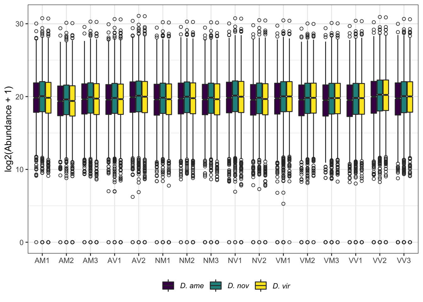
Load Orthofinder results
# OrthoFinder orthogroups output
orthogroups <- read_tsv('../TPP_aalysis/orthofinder/Results_Sep13/Orthogroups/Orthogroups.tsv')

## omit NAs as we are only interseted in reciprocal 1:1:1 between all species
orthogroup_long <- na.omit(orthogroups) %>%
  pivot_longer(cols = 2:4) %>%
  separate_rows(value, sep = ", ") %>%
  rename(protein = value, species = name)

# percentage of all proteins assigned to orthogroups
orthogroup_long %>%
  group_by(species) %>%
  count() %>%
  # add total numbers of proteins in each proteome
  #bind_cols(N = c(11958, 12729, 12792)) %>%
  # or n_distinct orthogroups
  bind_cols(N = n_distinct(orthogroups$Orthogroup)) %>%
  mutate(prop.orth = n/N)
# A tibble: 3 × 4
# Groups: species [3]
species n N prop.orth
<chr> <int> <int> <dbl>
1 Dame 8281 10777 0.768
2 Dnov 7878 10777 0.731
3 Dvir 7956 10777 0.738og_counts <- orthogroup_long %>%
group_by(species, Orthogroup) %>%
count(name = "N") %>%
mutate(orth_numb = as.numeric(str_sub(Orthogroup, 3))) %>%
ungroup()
# count numbers of proteins by orthogroup
og_counts %>%
group_by(species, N) %>%
count() %>% #filter(N > 1) %>%
mutate(N2 = ifelse(N > 4, "5+", as.character(N)),
n2 = ifelse(N == 1, n/7, n)) %>%
ggplot(aes(x = N2, y = n2, fill = species)) +
geom_bar(stat = "identity", position = "dodge") +
scale_fill_viridis_d()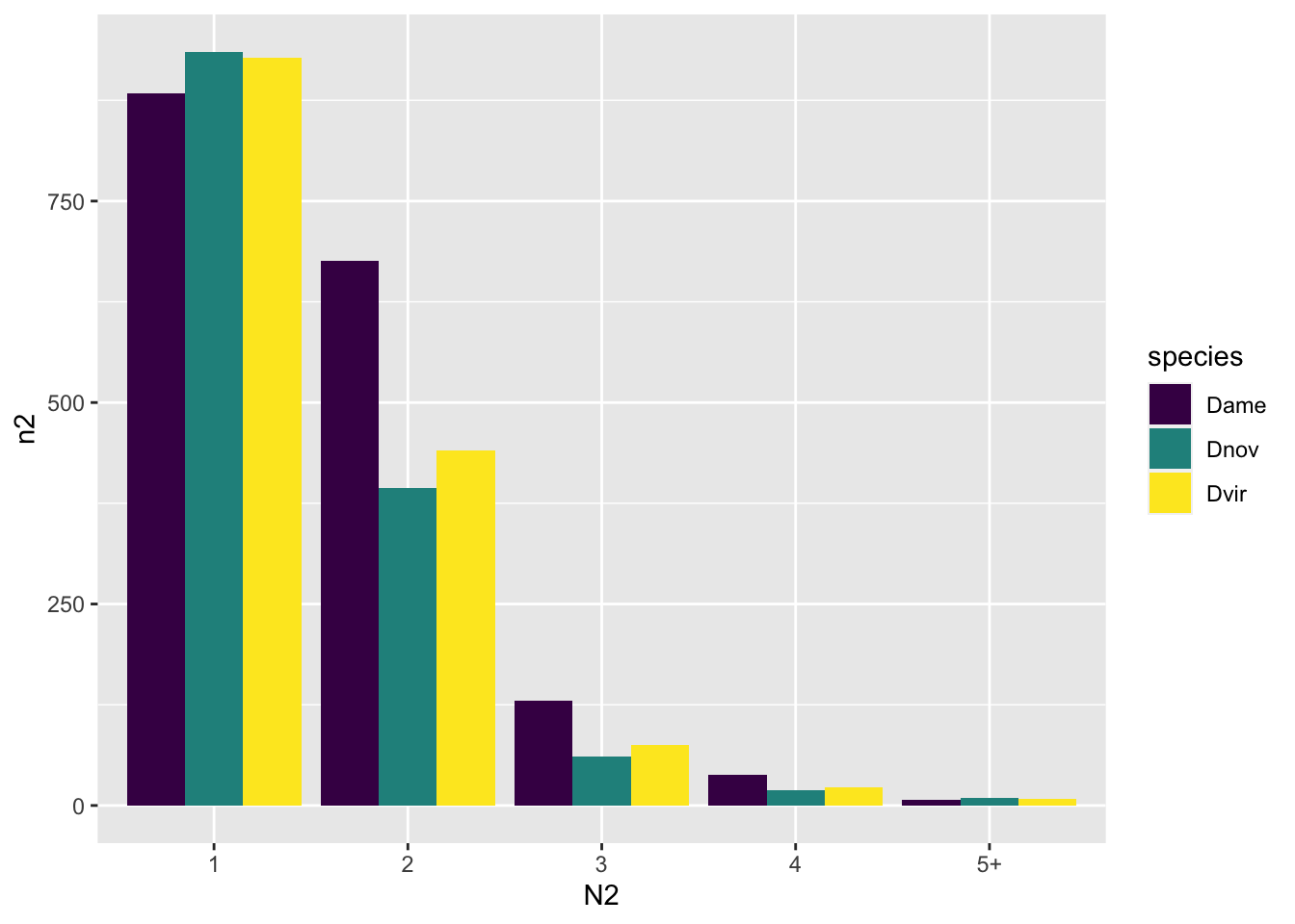
Load signal peptides predictions
We submitted each species proteome to Phobius and ran SignalP-5.0 locally to identify predicted signal peptide sequences and then combined the results.
# Phobius results
phob_ame <- read.delim('../TPP_aalysis/DameSB_db/phobius.txt') %>%
  dplyr::rename(protein = SEQENCE.ID)
phob_nov <- read.delim('../TPP_aalysis/Dnov14_db/phobius.txt') %>%
  dplyr::rename(protein = SEQENCE.ID)
phob_vir <- read.delim('../TPP_aalysis/Dvir87_db/phobius.txt') %>%
  dplyr::rename(protein = SEQENCE.ID)

# SigP/Trinotate results
ame_sigp <- read.csv('../TPP_aalysis/DameSB_db/Trinotate_ame.csv') %>% filter(SignalP != '.') %>%
  rename(gene_id = X.gene_id) %>% distinct(gene_id) %>% pull(gene_id)

nov_sigp <- read.csv('../TPP_aalysis/Dnov14_db/Trinotate_nov.csv') %>% filter(SignalP != '.') %>%
  rename(gene_id = X.gene_id) %>% distinct(gene_id) %>% pull(gene_id)

vir_sigp <- read.csv('../TPP_aalysis/Dvir87_db/Trinotate_vir.csv') %>% filter(SignalP != '.') %>%
  rename(gene_id = X.gene_id) %>% distinct(gene_id) %>% pull(gene_id)

# #overlap between methods
# upset(fromList(list(
#   Phobius = phob_vir %>%
#     filter(SP == 'Y') %>% pull(protein),
#   SignalP = vir_sigp)))

# combine results
signal_peps_ame <- combine(phob_ame %>% filter(SP == 'Y') %>% pull(protein),
                           ame_sigp) %>% unique()

signal_peps_nov <- combine(phob_nov %>% filter(SP == 'Y') %>% pull(protein),
                           nov_sigp) %>% unique()

signal_peps_vir <- combine(phob_vir %>% filter(SP == 'Y') %>% pull(protein),
                           vir_sigp) %>% unique()

# add orthogroup ID
ame_sig <- data.frame(protein = signal_peps_ame) %>%
  left_join(orthogroup_long %>% filter(species == "Dame"), by = "protein", na_matches = "never")

nov_sig <- data.frame(protein = signal_peps_nov) %>%
  left_join(orthogroup_long %>% filter(species == "Dnov"), by = "protein", na_matches = "never")

vir_sig <- data.frame(protein = signal_peps_vir) %>%
  left_join(orthogroup_long %>% filter(species == "Dvir"), by = "protein", na_matches = "never")
Load other data
vir_ids <- read.delim('data/virilis_molecular_evolution_results/gffread_annotated_transcripts.gene_trans_map',
                      header = FALSE) %>%
  dplyr::rename(FBgn = V1,
                FBtr = V2)

# virilis group AG/SFP/EB biased genes
Dvir_SFPs <- read.delim('data/virilis_male_AG_SFP_EB_genes.txt', header = FALSE) %>%
  dplyr::rename(bias = V1,
                FBgn = V2)

# Dmel sperm proteome orthologs
sperm_mel <- inner_join(
  # Dmel Sperm proteome II (Wasbrough et al. 2010 J. Prot.)
  read.csv('data/melanogaster/DmSPii_Supp.Table3.csv'),
  # melanogaster orthologs
  read.table(file = "data/melanogaster/mel_orths.txt", header = T),
  by = c('Gene.Symbol' = 'mel_GeneSymbol')) %>%
  select(FBgn_v = FBgn_ID, mel_FBgn_ID, Gene.Name, Gene.Symbol, mel_Arm) %>%
  left_join(vir_ids, by = c('FBgn_v' = 'FBgn'), na_matches = "never") %>%
  distinct(FBgn_v, .keep_all = TRUE)

# Dmel SFP orthologs
wigbySFP <- inner_join(
  # List of SFPs (Wigby et al. 2020 Phil. Trans. B.)
  read.csv('data/melanogaster/dmel_SFPs_wigby_etal2020.csv') %>%
  filter(category == 'highconf'),
  # melanogaster orthologs
  read.table(file = "data/melanogaster/mel_orths.txt", header = T),
  by = c('FBgn' = 'mel_FBgn_ID'), na_matches = "never") %>%
  select(FBgn = FBgn_ID, FBgn_mel = FBgn, Symbol) %>%
  left_join(vir_ids, by = c('FBgn'), na_matches = "never") %>%
  distinct(FBgn, .keep_all = TRUE)

# Ahmed-Braimah et al. 2020 MBE data
# virilis gene FBgns FRT biased genes
FRTbiased <- readxl::read_excel('data/ABetal.2020/File_S1.xlsx')
# virilis gene FBgns changing in expression after mating
virilisPMDE <- readxl::read_excel('data/ABetal.2020/File_S3.xlsx')

# pairwise Ka.Ks values
kaks_results <- read.delim('data/virilis_molecular_evolution_results/KaKs.ALL.results.txt') %>%
  left_join(vir_ids, by = c('FBtr_ID' = 'FBtr'), na_matches = "never")

# FlyBase GO terms
flybase_GO <- read.delim('data/FlyBase_GO_STEP.txt') %>%
  dplyr::rename(FBgn = X.SUBMITTED.ID) %>%
  # merge Dmel orthologs and IDs
  left_join(read.table(file = "data/melanogaster/mel_orths.txt", header = T),
            by = c('FBgn' = 'FBgn_ID'), na_matches = "never") %>%
  distinct(FBgn, .keep_all = TRUE)

# All genes with annotation including 'serin' from FlyBase
STEP <- flybase_GO %>%
  filter(stringr::str_detect(GO_BIOLOGICAL_PROCESS, 'serin') |
           stringr::str_detect(GO_MOLECULAR_FUNCTION, 'serin'))
get gene ids and orthologs
# Add D. virilis FBgns Ids
ame_fbgn <- read.csv('../TPP_aalysis/DameSB_db/Trinotate_ame.csv') %>%
  mutate(FBtr = gsub('\\^.*', '', x = dvir.proteins.fasta_BLASTX)) %>%
  select(gene_id = X.gene_id, FBtr) %>%
  left_join(vir_ids %>% select(FBtr, FBgn), na_matches = "never") %>%
  distinct(gene_id, FBgn, FBtr) %>% filter(FBtr != '.') %>%
  left_join(orthogroup_long %>% filter(species == 'Dame') %>%
              select(Orthogroup, protein),
            by = c('gene_id' = 'protein'), na_matches = "never")

nov_fbgn <- read.csv('../TPP_aalysis/Dnov14_db/Trinotate_nov.csv') %>%
  mutate(FBtr = gsub('\\^.*', '', x = dvir.proteins.fasta_BLASTX)) %>%
  select(gene_id = X.gene_id, FBtr) %>%
  left_join(vir_ids %>% select(FBtr, FBgn), na_matches = "never") %>%
  distinct(gene_id, FBgn, FBtr) %>% filter(FBtr != '.') %>%
  left_join(orthogroup_long %>% filter(species == 'Dnov') %>%
              select(Orthogroup, protein),
            by = c('gene_id' = 'protein'), na_matches = "never")

vir_fbgn <- read.csv('../TPP_aalysis/Dvir87_db/Trinotate_vir.csv') %>%
  mutate(FBtr = gsub('\\^.*', '', x = dvir.proteins.fasta_BLASTX)) %>%
  select(gene_id = X.gene_id, FBtr) %>%
  left_join(vir_ids %>% select(FBtr, FBgn), na_matches = "never") %>%
  distinct(gene_id, FBgn, FBtr) %>% filter(FBtr != '.') %>%
  left_join(orthogroup_long %>% filter(species == 'Dvir') %>%
              select(Orthogroup, protein),
            by = c('gene_id' = 'protein'), na_matches = "never")
Differential abundance analysis
Single species database analysis
Identifying ejaculate candidates
We performed differential abundance analysis between mated and virgin samples for each species, and between species, using each species database. We considered proteins as differentially abundant based on an adjusted p-value < 0.05 and logFC > |1|.
# filter 2 unique peptides and replace blanks (NA's) with 0's
ame_abund <- tmt_ame_prot %>% filter(UP >= 2) %>% mutate(across(3:18, ~replace_na(.x, 0)))
nov_abund <- tmt_nov_prot %>% filter(UP >= 2) %>% mutate(across(3:18, ~replace_na(.x, 0)))
vir_abund <- tmt_vir_prot %>% filter(UP >= 2) %>% mutate(across(3:18, ~replace_na(.x, 0)))

# get sample info - same for all db's
sampInfo = data.frame(condition = str_sub(colnames(ame_abund[-c(1, 2)]), 1, 2),
                      Replicate = str_sub(colnames(ame_abund[-c(1, 2)]), 3, 3))

# make design matrix to test diffs between groups
design <- model.matrix(~0 + sampInfo$condition)
colnames(design) <- unique(sampInfo$condition)
rownames(design) <- sampInfo$Replicate

# make contrasts - higher values = higher in mated
cont.matrix <- makeContrasts(M.a.V = AM - AV,
                             M.n.V = NM - NV,
                             M.v.V = VM - VV,
                             levels = design)

# create DGElist
dge_ame <- DGEList(counts = ame_abund[, -c(1, 2)], genes = ame_abund$protein, group = sampInfo$condition)
dge_nov <- DGEList(counts = nov_abund[, -c(1, 2)], genes = nov_abund$protein, group = sampInfo$condition)
dge_vir <- DGEList(counts = vir_abund[, -c(1, 2)], genes = vir_abund$protein, group = sampInfo$condition)

# ## Remove rows consistently have zero or very low counts
# keep_ame <- filterByExpr(dge_ame)
# keep_nov <- filterByExpr(dge_nov)
# keep_vir <- filterByExpr(dge_vir)

keep_ame <- rowSums(cpm(dge_ame) > 1) >= 8
keep_nov <- rowSums(cpm(dge_nov) > 1) >= 8
keep_vir <- rowSums(cpm(dge_vir) > 1) >= 8

dge_ame <- dge_ame[keep_ame, keep.lib.sizes = FALSE]
dge_nov <- dge_nov[keep_nov, keep.lib.sizes = FALSE]
dge_vir <- dge_vir[keep_vir, keep.lib.sizes = FALSE]

dge_ame <- calcNormFactors(dge_ame, method = 'TMM')
dge_nov <- calcNormFactors(dge_nov, method = 'TMM')
dge_vir <- calcNormFactors(dge_vir, method = 'TMM')

dge_ame <- estimateCommonDisp(dge_ame)
dge_nov <- estimateCommonDisp(dge_nov)
dge_vir <- estimateCommonDisp(dge_vir)

dge_ame <- estimateTagwiseDisp(dge_ame)
dge_nov <- estimateTagwiseDisp(dge_nov)
dge_vir <- estimateTagwiseDisp(dge_vir)

# voom normalisation
dge_ameV <- voom(dge_ame, design, plot = FALSE)
dge_novV <- voom(dge_nov, design, plot = FALSE)
dge_virV <- voom(dge_vir, design, plot = FALSE)

# fit linear model
lm_ame <- lmFit(dge_ameV, design = design)
lm_nov <- lmFit(dge_novV, design = design)
lm_vir <- lmFit(dge_virV, design = design)
Diagnostic plots
diag_plot <- function(dgelist = NA, design = NA) {

  par(mfrow = c(2,2))
  # Biological coefficient of variation
  plotBCV(dgelist)
  # mean-variance trend
  voomed = voom(dgelist, design, plot = TRUE)
  # QQ-plot
  g <- gof(glmFit(dgelist, design))
  z <- zscoreGamma(g$gof.statistics,shape = g$df/2,scale = 2)
  qqnorm(z); qqline(z, col = 4,lwd = 1,lty = 1)
  # log2 transformed and normalize boxplot of counts across samples
  boxplot(voomed$E, xlab = "", ylab = "log2(Abundance)", las = 2, main = "Voom transformed logCPM",
          col = c(rep(2:7, c(3, 2, 3, 2, 3, 3))))
  abline(h = median(voomed$E), col = "blue")
  par(mfrow = c(1,1))

}
ame.db
diag_plot(dge_ame, design)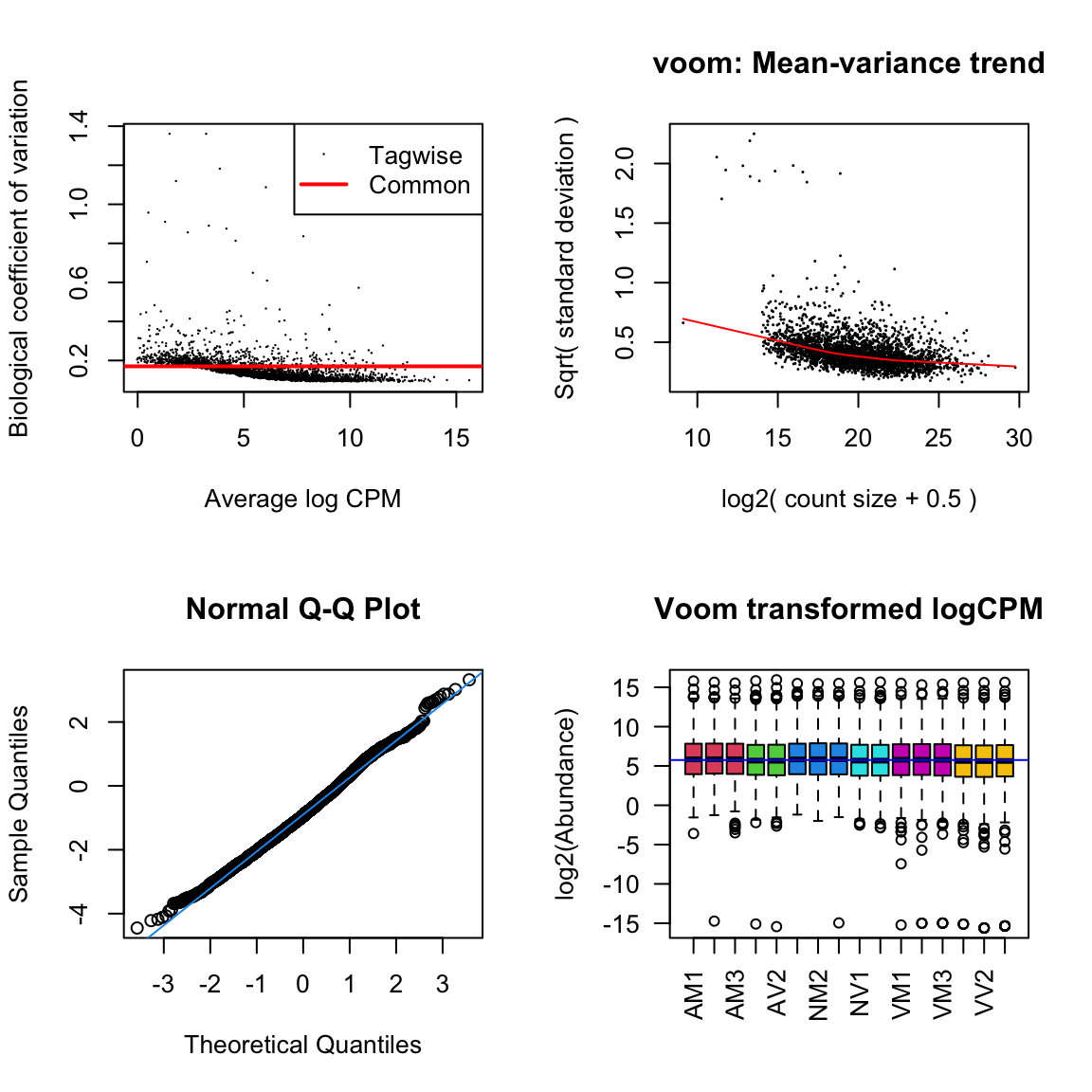
nov.db
diag_plot(dge_nov, design)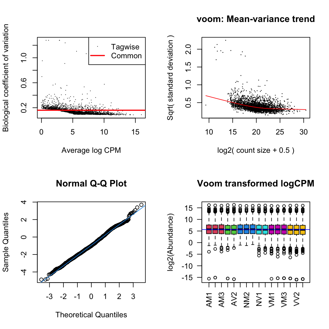
vir.db
diag_plot(dge_vir, design)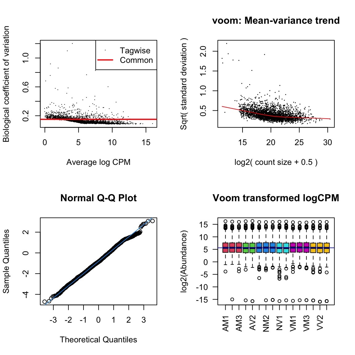
compare DA between mated/virgin
# ame using each database
lm_ame2ame <- contrasts.fit(lm_ame, cont.matrix[,"M.a.V"])
lm_ame2nov <- contrasts.fit(lm_nov, cont.matrix[,"M.a.V"])
lm_ame2vir <- contrasts.fit(lm_vir, cont.matrix[,"M.a.V"])

lm_ame2ame <- eBayes(lm_ame2ame)
lm_ame2nov <- eBayes(lm_ame2nov)
lm_ame2vir <- eBayes(lm_ame2vir)

lm_ame2ame.tTags.table <- topTable(lm_ame2ame, adjust.method = "BH", number = Inf)
lm_ame2nov.tTags.table <- topTable(lm_ame2nov, adjust.method = "BH", number = Inf)
lm_ame2vir.tTags.table <- topTable(lm_ame2vir, adjust.method = "BH", number = Inf)

# nov using each database
lm_nov2ame <- contrasts.fit(lm_ame, cont.matrix[,"M.n.V"])
lm_nov2nov <- contrasts.fit(lm_nov, cont.matrix[,"M.n.V"])
lm_nov2vir <- contrasts.fit(lm_vir, cont.matrix[,"M.n.V"])

lm_nov2ame <- eBayes(lm_nov2ame)
lm_nov2nov <- eBayes(lm_nov2nov)
lm_nov2vir <- eBayes(lm_nov2vir)

lm_nov2ame.tTags.table <- topTable(lm_nov2ame, adjust.method = "BH", number = Inf)
lm_nov2nov.tTags.table <- topTable(lm_nov2nov, adjust.method = "BH", number = Inf)
lm_nov2vir.tTags.table <- topTable(lm_nov2vir, adjust.method = "BH", number = Inf)

# vir using each database
lm_vir2ame <- contrasts.fit(lm_ame, cont.matrix[,"M.v.V"])
lm_vir2nov <- contrasts.fit(lm_nov, cont.matrix[,"M.v.V"])
lm_vir2vir <- contrasts.fit(lm_vir, cont.matrix[,"M.v.V"])

lm_vir2ame <- eBayes(lm_vir2ame)
lm_vir2nov <- eBayes(lm_vir2nov)
lm_vir2vir <- eBayes(lm_vir2vir)

lm_vir2ame.tTags.table <- topTable(lm_vir2ame, adjust.method = "BH", number = Inf)
lm_vir2nov.tTags.table <- topTable(lm_vir2nov, adjust.method = "BH", number = Inf)
lm_vir2vir.tTags.table <- topTable(lm_vir2vir, adjust.method = "BH", number = Inf)

# combine results
ame_DATABLES <- rbind(lm_ame2ame.tTags.table %>% mutate(species = 'ame'),
                      lm_nov2ame.tTags.table %>% mutate(species = 'nov'),
                      lm_vir2ame.tTags.table %>% mutate(species = 'vir')) %>%
  mutate(DB = 'ame.db',
         threshold = if_else(adj.P.Val < 0.05 & abs(logFC) > 1, 'DA', 'NS'),
         # add variable for signal peptides reaching significance threshold
         sigP = case_when(genes %in% ame_sig$protein & threshold == 'DA' ~ 'sigP',
                          threshold == 'DA' ~ 'DA',
                          TRUE ~ 'NS'),
         # add variable splitting by bias to virgin vs. mated and signal peptide
         DA = case_when(genes %in% ame_sig$protein & adj.P.Val < 0.05 & logFC > 1 ~ "MBsec",
                        genes %in% ame_sig$protein & adj.P.Val < 0.05 & logFC < -1 ~ "FMsec",
                        adj.P.Val < 0.05 & logFC > 1 ~ "MB",
                        adj.P.Val < 0.05 & logFC < -1 ~ "FM",
                        TRUE ~ 'NS')) %>%
  # add orthologs
  left_join(orthogroup_long %>% filter(species == "Dame") %>% select(-species), by = c("genes" = "protein"), na_matches = "never")

nov_DATABLES <- rbind(lm_ame2nov.tTags.table %>% mutate(species = 'ame'),
                      lm_nov2nov.tTags.table %>% mutate(species = 'nov'),
                      lm_vir2nov.tTags.table %>% mutate(species = 'vir')) %>%
  mutate(DB = 'nov.db',
         threshold = if_else(adj.P.Val < 0.05 & abs(logFC) > 1, 'DA', 'NS'),
         # add variable for signal peptides reaching significance threshold
         sigP = case_when(genes %in% nov_sig$protein & threshold == 'DA' ~ 'sigP',
                          threshold == 'DA' ~ 'DA',
                          TRUE ~ 'NS'),
         # add variable splitting by bias to virgin vs. mated and signal peptide
         DA = case_when(genes %in% nov_sig$protein & adj.P.Val < 0.05 & logFC > 1 ~ "MBsec",
                        genes %in% nov_sig$protein & adj.P.Val < 0.05 & logFC < -1 ~ "FMsec",
                        adj.P.Val < 0.05 & logFC > 1 ~ "MB",
                        adj.P.Val < 0.05 & logFC < -1 ~ "FM",
                        TRUE ~ 'NS')) %>%
  # add orthologs
  left_join(orthogroup_long %>% filter(species == "Dnov") %>% select(-species), by = c("genes" = "protein"), na_matches = "never")

vir_DATABLES <- rbind(lm_ame2vir.tTags.table %>% mutate(species = 'ame'),
                      lm_nov2vir.tTags.table %>% mutate(species = 'nov'),
                      lm_vir2vir.tTags.table %>% mutate(species = 'vir')) %>%
  mutate(DB = 'vir.db',
         threshold = if_else(adj.P.Val < 0.05 & abs(logFC) > 1, 'DA', 'NS'),
         # add variable for signal peptides reaching significance threshold
         sigP = case_when(genes %in% vir_sig$protein & threshold == 'DA' ~ 'sigP',
                          threshold == 'DA' ~ 'DA',
                          TRUE ~ 'NS'),
         # add variable splitting by bias to virgin vs. mated and signal peptide
         DA = case_when(genes %in% vir_sig$protein & adj.P.Val < 0.05 & logFC > 1 ~ "MBsec",
                        genes %in% vir_sig$protein & adj.P.Val < 0.05 & logFC < -1 ~ "FMsec",
                        adj.P.Val < 0.05 & logFC > 1 ~ "MB",
                        adj.P.Val < 0.05 & logFC < -1 ~ "FM",
                        TRUE ~ 'NS')) %>%
  # add orthologs
  left_join(orthogroup_long %>% filter(species == "Dvir") %>% select(-species), by = c("genes" = "protein"), na_matches = "never")
Volcano plots
# plot all vs. all
bind_rows(ame_DATABLES,
          nov_DATABLES,
          vir_DATABLES) %>%
  ggplot(aes(x = logFC, y = -log10(adj.P.Val), colour = DA)) +
  geom_point(alpha = .6) +
  scale_colour_manual(values = c('hotpink', 'red', 'blue', 'purple', 'grey40')) +
  labs(y = '-log10(p-value)') +
  facet_grid(species ~ DB) +
  theme_bw() +
  theme(legend.position = 'bottom',
        legend.title = element_blank(),
        legend.background = element_rect(fill = NA)) +
  #ggsave('plots/database_comps/volcano_mated-virgin_all.vs.all.pdf', height = 17.8, width = 17.8, units = 'cm', dpi = 600, useDingbats = FALSE) +
  NULL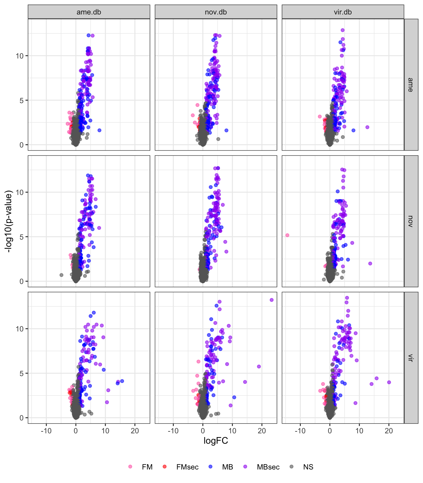
Plot species specific database
facet_names <- c(ame = "D. americana",
                 nov = 'D. novamexicana',
                 vir = "D. virilis")

lab_text <- data.frame(species = c('ame', 'nov', 'vir'),
                       P.Value = min(nov_DATABLES$P.Value),
                       logFC = 20,
                       lab = c("D. americana", 'D. novamexicana', "D. virilis"),
                       DA = NA,
                       threshold = NA)

# plot
bind_rows(ame_DATABLES %>% filter(species == 'ame'),
          nov_DATABLES %>% filter(species == 'nov'),
          vir_DATABLES %>% filter(species == 'vir')) %>%
  ggplot(aes(x = logFC, y = -log10(P.Value), colour = DA, shape = threshold)) +
  geom_point(alpha = .6) +
  scale_shape_manual(values = c(16, 1), guide = 'none') +
  scale_colour_manual(values = c(egypt.pal[4:1], "grey60")) +
  labs(y = '-log10(p-value)') +
  facet_wrap(~species, nrow = 1, labeller = as_labeller(facet_names)) +
  theme_bw() +
  theme(legend.position = '',#c(0.04, 0.8),
        legend.title = element_blank(),
        legend.background = element_rect(fill = NA),
        strip.text = element_text(size = 15, face = "italic"),
        strip.background = element_blank(),
        strip.text.x = element_blank()) +
  geom_text(data = lab_text, colour = 'black', hjust = 1,
            aes(y = -log10(P.Value), label = paste0(lab)), size = 4, fontface = "italic") +
  #ggsave('plots/TPP_volcano_mated-virgin.pdf', height = 7, width = 19, units = 'cm', dpi = 600, useDingbats = FALSE) +
  NULL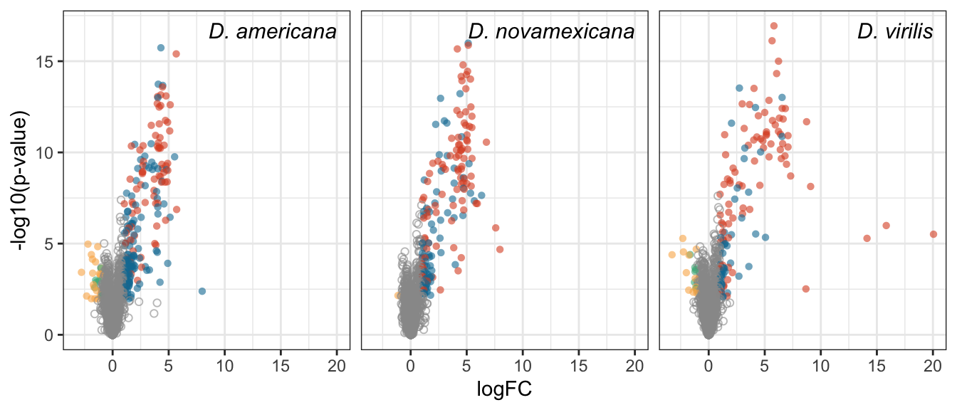
Overlap in ‘Sfps’ between species
We compare the numbers of ejaculate candidates detected using each species database.
ame db
# subset only higher in mated
ame_cands <- ame_DATABLES %>% filter(str_detect(DA, pattern = 'MB'))

# # overlap for ejaculate candidates with orthologs using each database
# upset(fromList(list(ame = split(ame_cands, ame_cands$species)[[1]][[1]],
#                     nov = split(ame_cands, ame_cands$species)[[2]][[1]],
#                     vir = split(ame_cands, ame_cands$species)[[3]][[1]])))

plot(euler(c('ame' = 50, "nov" = 22, "vir" = 26,
             'ame&nov' = 51, 'ame&vir' = 16, 'nov&vir' = 0,
             'ame&nov&vir' = 92)),
     quantities = TRUE,
     fills = list(fill = viridis::viridis(n = 3), alpha = .5))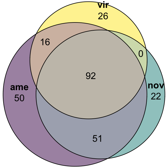
nov db
# subset only higher in mated
nov_cands <- nov_DATABLES %>% filter(str_detect(DA, pattern = 'MB'))

# # overlap for ejaculate candidates with orthologs using each database
# upset(fromList(list(ame = split(nov_cands, nov_cands$species)[[1]][[1]],
#                     nov = split(nov_cands, nov_cands$species)[[2]][[1]],
#                     vir = split(nov_cands, nov_cands$species)[[3]][[1]])))

plot(euler(c('ame' = 40, "nov" = 22, "vir" = 27,
             'ame&nov' = 56, 'ame&vir' = 10, 'nov&vir' = 3,
             'ame&nov&vir' = 104)),
     quantities = TRUE,
     fills = list(fill = viridis::viridis(n = 3), alpha = .5))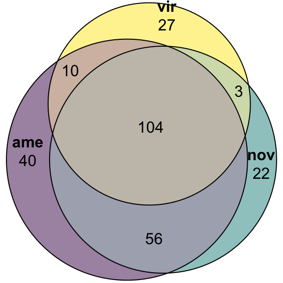
vir db
# subset only higher in mated
vir_cands <- vir_DATABLES %>% filter(str_detect(DA, pattern = 'MB'))

# # overlap for ejaculate candidates with orthologs using each database
# upset(fromList(list(ame = split(vir_cands, vir_cands$species)[[1]][[1]],
#                     nov = split(vir_cands, vir_cands$species)[[2]][[1]],
#                     vir = split(vir_cands, vir_cands$species)[[3]][[1]])))

plot(euler(c('ame' = 34, "nov" = 25, "vir" = 19,
             'ame&nov' = 41, 'ame&vir' = 18, 'nov&vir' = 2,
             'ame&nov&vir' = 91)),
     quantities = TRUE,
     fills = list(fill = viridis::viridis(n = 3), alpha = .5))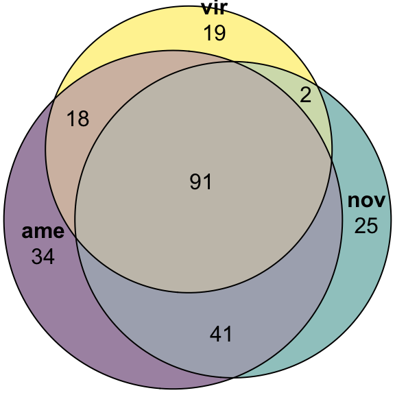
# combine ejaculate candidates
ejac_cands <- bind_rows(ame_cands %>% left_join(ame_fbgn, by = c("genes" = "gene_id", "Orthogroup")),
                        nov_cands %>% left_join(nov_fbgn, by = c("genes" = "gene_id", "Orthogroup")),
                        vir_cands %>% left_join(vir_fbgn, by = c("genes" = "gene_id", "Orthogroup"))) %>%
  distinct(genes, species, DB, Orthogroup, .keep_all = TRUE)

# # overlap for ejaculate candidates with orthologs using each database
# upset(fromList(list(ame.db = split(ejac_cands, ejac_cands$DB)[[1]][[13]],
#                     nov.db = split(ejac_cands, ejac_cands$DB)[[2]][[13]],
#                     vir.db = split(ejac_cands, ejac_cands$DB)[[3]][[13]])))

plot(venn(c('D. ame' = 39, 'D. nov' = 34, 'D. vir' = 26,
            'D. ame&D. nov' = 20, 'D. ame&D. vir' = 12, 'D. nov&D. vir' = 36,
            'D. ame&D. nov&D. vir' = 118)),
     quantities = TRUE,
     fills = list(fill = viridis::viridis(n = 3), alpha = .5))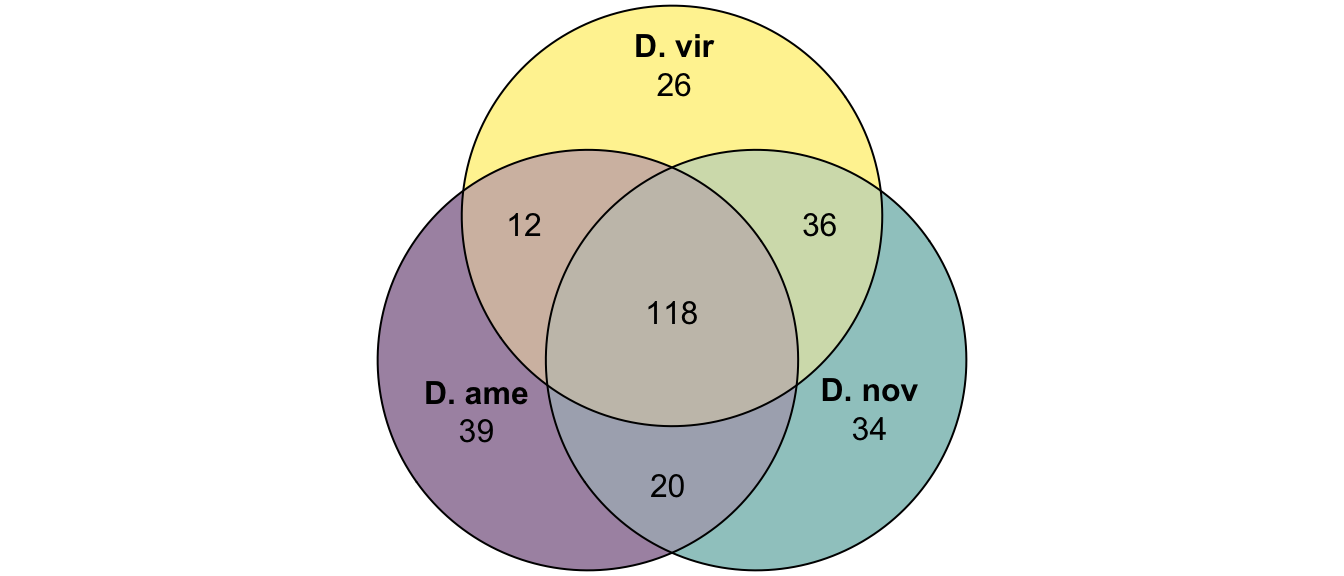
# overlap in ejaculate candidates between species
ejac_cands %>%
  mutate(orth = if_else(is.na(Orthogroup) == TRUE, 'no', 'yes')) %>%
  group_by(DB, orth) %>%
  summarise(N = n_distinct(genes)) %>%
  pivot_wider(id_cols = DB, names_from = orth, values_from = N) %>%
  mutate(total = yes + no,
         prop.orths = yes/total) %>%
  kable(digits = 3,
        caption = 'Numbers and proportions of ejaculate candidates in each species with or without orthologs') %>%
kable_styling(full_width = FALSE)| DB | no | yes | total | prop.orths |
|---|---|---|---|---|
| ame.db | 60 | 197 | 257 | 0.767 |
| nov.db | 51 | 211 | 262 | 0.805 |
| vir.db | 35 | 195 | 230 | 0.848 |
# # write file of all distinct proteins with/out 1:1:1 orthologs
# ejac_cands %>%
#   mutate(orth = if_else(is.na(Orthogroup) == TRUE, 'no', 'yes')) %>%
#   #write_csv('output/ClueGOlists/all_ejac_IDs.csv')
#   filter(orth == "no") %>%
#   distinct(genes, DB) %>%
#   write_csv('output/ClueGOlists/ejac_IDs_no-orths.csv')

#number of ejaculate candidates using each species database including without orthologs
ejac_ids <- bind_rows(ame_DATABLES %>% filter(str_detect(DA, pattern = 'MB')),
                      nov_DATABLES %>% filter(str_detect(DA, pattern = 'MB')),
                      vir_DATABLES %>% filter(str_detect(DA, pattern = 'MB'))) %>%
  mutate(OrthID = if_else(is.na(Orthogroup) == TRUE, paste0(genes, "-", species), Orthogroup)) %>%
  distinct(genes, DB, .keep_all = TRUE) #%>% drop_na(Orthogroup)

# total number of unique ejaculate candidates identified
#n_distinct(ejac_ids$OrthID)

# upset(fromList(list(ame = split(ejac_ids, ejac_ids$DB)[[1]][[14]],
#                     nov = split(ejac_ids, ejac_ids$DB)[[2]][[14]],
#                     vir = split(ejac_ids, ejac_ids$DB)[[3]][[14]])))

#pdf('plots/sfp_overlap_all_db_noOrths.pdf', height = 4, width = 4)
plot(venn(c('D. ame' = 99, 'D. nov' = 85, 'D. vir' = 61,
            'D. ame&D. nov' = 20, 'D. ame&D. vir' = 12, 'D. nov&D. vir' = 36,
            'D. ame&D. nov&D. vir' = 117)
          ),
     quantities = TRUE,
     fills = list(fill = viridis::viridis(n = 3), alpha = .5))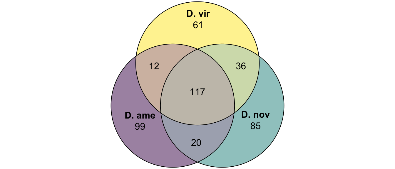
#dev.off()

# number and proportion secreted
bind_rows(ame_DATABLES %>% filter(str_detect(DA, pattern = 'MB')),
          nov_DATABLES %>% filter(str_detect(DA, pattern = 'MB')),
          vir_DATABLES %>% filter(str_detect(DA, pattern = 'MB'))) %>%
  distinct(genes, DB, .keep_all = TRUE) %>%
  group_by(DB, DA) %>% dplyr::count() %>%
  pivot_wider(id_cols = DB, names_from = DA, values_from = n) %>%
  mutate(prop.sec = MBsec/(MBsec + MB)) %>%
  kable(digits = 3,
        caption = 'The number of proteins higher in abundance in mated comapred to virgin samples with or without a secretion signal using each species database') %>%
kable_styling(full_width = FALSE)| DB | MB | MBsec | prop.sec |
|---|---|---|---|
| ame.db | 161 | 96 | 0.374 |
| nov.db | 126 | 136 | 0.519 |
| vir.db | 103 | 127 | 0.552 |
# #write FBgns for ClueGO - ejaculate candidates
# ejac_cands %>% distinct(FBgn, .keep_all = TRUE) %>%
#   write_csv('output/ClueGOlists/TPP_all_ejac_FBgn.csv')

# # proteins higher abundance in FRT
# bind_rows(ame_DATABLES %>% filter(str_detect(DA, pattern = 'FM')) %>%
#             left_join(ame_fbgn, by = c("genes" = "gene_id", "Orthogroup")),
#           nov_DATABLES %>% filter(str_detect(DA, pattern = 'FM')) %>%
#             left_join(nov_fbgn, by = c("genes" = "gene_id", "Orthogroup")),
#           vir_DATABLES %>% filter(str_detect(DA, pattern = 'FM')) %>%
#             left_join(vir_fbgn, by = c("genes" = "gene_id", "Orthogroup"))) %>%
#   distinct(genes, species, DB, Orthogroup, .keep_all = TRUE) %>%
#   write_csv('output/ClueGOlists/TPP_virgin_biased_FBgn.csv')
Divergence between ejaculate candidates
Here we perform pairwise differential abundance analysis between species for mated samples only to identify differences in the male ejaculate between species. We subset the data to include only ‘ejaculate candidates’ - i.e. proteins significantly higher abundance in mated compared to virgin samples. We performed analyses using each species database.
# subset data to only include ejaculate candidates
ame_mated <- ame_abund %>% dplyr::select(protein, contains('M')) %>%
  filter(protein %in% ejac_cands$genes[ejac_cands$DB == 'ame.db'])

nov_mated <- nov_abund %>% dplyr::select(protein, contains('M')) %>%
  filter(protein %in% ejac_cands$genes[ejac_cands$DB == 'nov.db'])

vir_mated <- vir_abund %>% dplyr::select(protein, contains('M')) %>%
  filter(protein %in% ejac_cands$genes[ejac_cands$DB == 'vir.db'])

# get sample info - same for all db's
sampInfo.m <- data.frame(condition = str_sub(colnames(ame_mated[2:10]), 1, 2),
                         Replicate = str_sub(colnames(ame_mated[2:10]), 3, 3))

# make design matrix to test diffs between groups
design.m <- model.matrix(~0 + sampInfo.m$condition)
colnames(design.m) <- unique(sampInfo.m$condition)
rownames(design.m) <- sampInfo.m$Replicate

# make contrasts - higher values = higher in mated
cont.mated <- makeContrasts(a.m.n = AM - NM,
                            a.m.v = AM - VM,
                            n.m.v = NM - VM,
                            levels = design.m)

# create DGElist and fit model
dge_ame.m <- DGEList(counts = ame_mated[, 2:10], genes = ame_mated$protein, group = sampInfo.m$condition)
dge_nov.m <- DGEList(counts = nov_mated[, 2:10], genes = nov_mated$protein, group = sampInfo.m$condition)
dge_vir.m <- DGEList(counts = vir_mated[, 2:10], genes = vir_mated$protein, group = sampInfo.m$condition)

dge_ame.m <- calcNormFactors(dge_ame.m, method = 'TMM')
dge_nov.m <- calcNormFactors(dge_nov.m, method = 'TMM')
dge_vir.m <- calcNormFactors(dge_vir.m, method = 'TMM')

dge_ame.m <- estimateCommonDisp(dge_ame.m)
dge_nov.m <- estimateCommonDisp(dge_nov.m)
dge_vir.m <- estimateCommonDisp(dge_vir.m)

dge_ame.m <- estimateTagwiseDisp(dge_ame.m)
dge_nov.m <- estimateTagwiseDisp(dge_nov.m)
dge_vir.m <- estimateTagwiseDisp(dge_vir.m)

# voom normalisation
dge_ame.m <- voom(dge_ame.m, design.m, plot = FALSE)
dge_nov.m <- voom(dge_nov.m, design.m, plot = FALSE)
dge_vir.m <- voom(dge_vir.m, design.m, plot = FALSE)

# fit linear model
lm_ame.m <- lmFit(dge_ame.m, design = design.m)
lm_nov.m <- lmFit(dge_nov.m, design = design.m)
lm_vir.m <- lmFit(dge_vir.m, design = design.m)

# compare DA between mated samples

# ame using each database
mated_an2ame <- contrasts.fit(lm_ame.m, cont.mated[,"a.m.n"])
mated_an2nov <- contrasts.fit(lm_nov.m, cont.mated[,"a.m.n"])
mated_an2vir <- contrasts.fit(lm_vir.m, cont.mated[,"a.m.n"])

mated_an2ame <- eBayes(mated_an2ame)
mated_an2nov <- eBayes(mated_an2nov)
mated_an2vir <- eBayes(mated_an2vir)

mated_an2ame.tTags.table <- topTable(mated_an2ame, adjust.method = "BH", number = Inf)
mated_an2nov.tTags.table <- topTable(mated_an2nov, adjust.method = "BH", number = Inf)
mated_an2vir.tTags.table <- topTable(mated_an2vir, adjust.method = "BH", number = Inf)

# nov using each database
mated_av2ame <- contrasts.fit(lm_ame.m, cont.mated[,"a.m.v"])
mated_av2nov <- contrasts.fit(lm_nov.m, cont.mated[,"a.m.v"])
mated_av2vir <- contrasts.fit(lm_vir.m, cont.mated[,"a.m.v"])

mated_av2ame <- eBayes(mated_av2ame)
mated_av2nov <- eBayes(mated_av2nov)
mated_av2vir <- eBayes(mated_av2vir)

mated_av2ame.tTags.table <- topTable(mated_av2ame, adjust.method = "BH", number = Inf)
mated_av2nov.tTags.table <- topTable(mated_av2nov, adjust.method = "BH", number = Inf)
mated_av2vir.tTags.table <- topTable(mated_av2vir, adjust.method = "BH", number = Inf)

# vir using each database
mated_nv2ame <- contrasts.fit(lm_ame.m, cont.mated[,"n.m.v"])
mated_nv2nov <- contrasts.fit(lm_nov.m, cont.mated[,"n.m.v"])
mated_nv2vir <- contrasts.fit(lm_vir.m, cont.mated[,"n.m.v"])

mated_nv2ame <- eBayes(mated_nv2ame)
mated_nv2nov <- eBayes(mated_nv2nov)
mated_nv2vir <- eBayes(mated_nv2vir)

mated_nv2ame.tTags.table <- topTable(mated_nv2ame, adjust.method = "BH", number = Inf)
mated_nv2nov.tTags.table <- topTable(mated_nv2nov, adjust.method = "BH", number = Inf)
mated_nv2vir.tTags.table <- topTable(mated_nv2vir, adjust.method = "BH", number = Inf)

# combine results
ame_MATED <- rbind(mated_an2ame.tTags.table %>% mutate(comparison = 'ame.v.nov'),
                   mated_av2ame.tTags.table %>% mutate(comparison = 'ame.v.vir'),
                   mated_nv2ame.tTags.table %>% mutate(comparison = 'nov.v.vir')) %>%
  mutate(DB = 'ame.db',
         threshold = if_else(adj.P.Val < 0.05 & abs(logFC) > 1, 'DA', 'NS'),
         # add variable for signal peptides
         sigP = if_else(genes %in% ame_sig$protein, 'sigP', 'not'),
         DA = case_when(sigP == 'sigP' & threshold == 'DA' ~ 'sigP',
                        threshold == 'DA' ~ 'DA',
                        TRUE ~ 'NS'))

nov_MATED <- rbind(mated_an2nov.tTags.table %>% mutate(comparison = 'ame.v.nov'),
                   mated_av2nov.tTags.table %>% mutate(comparison = 'ame.v.vir'),
                   mated_nv2nov.tTags.table %>% mutate(comparison = 'nov.v.vir')) %>%
  mutate(DB = 'nov.db',
         threshold = if_else(adj.P.Val < 0.05 & abs(logFC) > 1, 'DA', 'NS'),
         # add variable for signal peptides
         sigP = if_else(genes %in% nov_sig$protein, 'sigP', 'not'),
         DA = case_when(sigP == 'sigP' & threshold == 'DA' ~ 'sigP',
                        threshold == 'DA' ~ 'DA',
                        TRUE ~ 'NS'))

vir_MATED <- rbind(mated_an2vir.tTags.table %>% mutate(comparison = 'ame.v.nov'),
                   mated_av2vir.tTags.table %>% mutate(comparison = 'ame.v.vir'),
                   mated_nv2vir.tTags.table %>% mutate(comparison = 'nov.v.vir')) %>%
  mutate(DB = 'vir.db',
         threshold = if_else(adj.P.Val < 0.05 & abs(logFC) > 1, 'DA', 'NS'),
         # add variable for signal peptides
         sigP = if_else(genes %in% vir_sig$protein, 'sigP', 'not'),
         DA = case_when(sigP == 'sigP' & threshold == 'DA' ~ 'sigP',
                        threshold == 'DA' ~ 'DA',
                        TRUE ~ 'NS'))
Compare results using each species database
Volcano plots all vs. all
bind_rows(ame_MATED,
          nov_MATED,
          vir_MATED) %>%
  ggplot(aes(x = logFC, y = -log10(adj.P.Val), colour = DA)) +
  geom_point(alpha = .6) +
  scale_colour_manual(values = c('hotpink', 'grey40', 'red')) +
  labs(y = '-log10(p-value)') +
  facet_grid(comparison ~ DB) +
  theme_bw() +
  theme(#legend.position = '',
        legend.title = element_blank(),
        legend.background = element_rect(fill = NA)) +
  NULL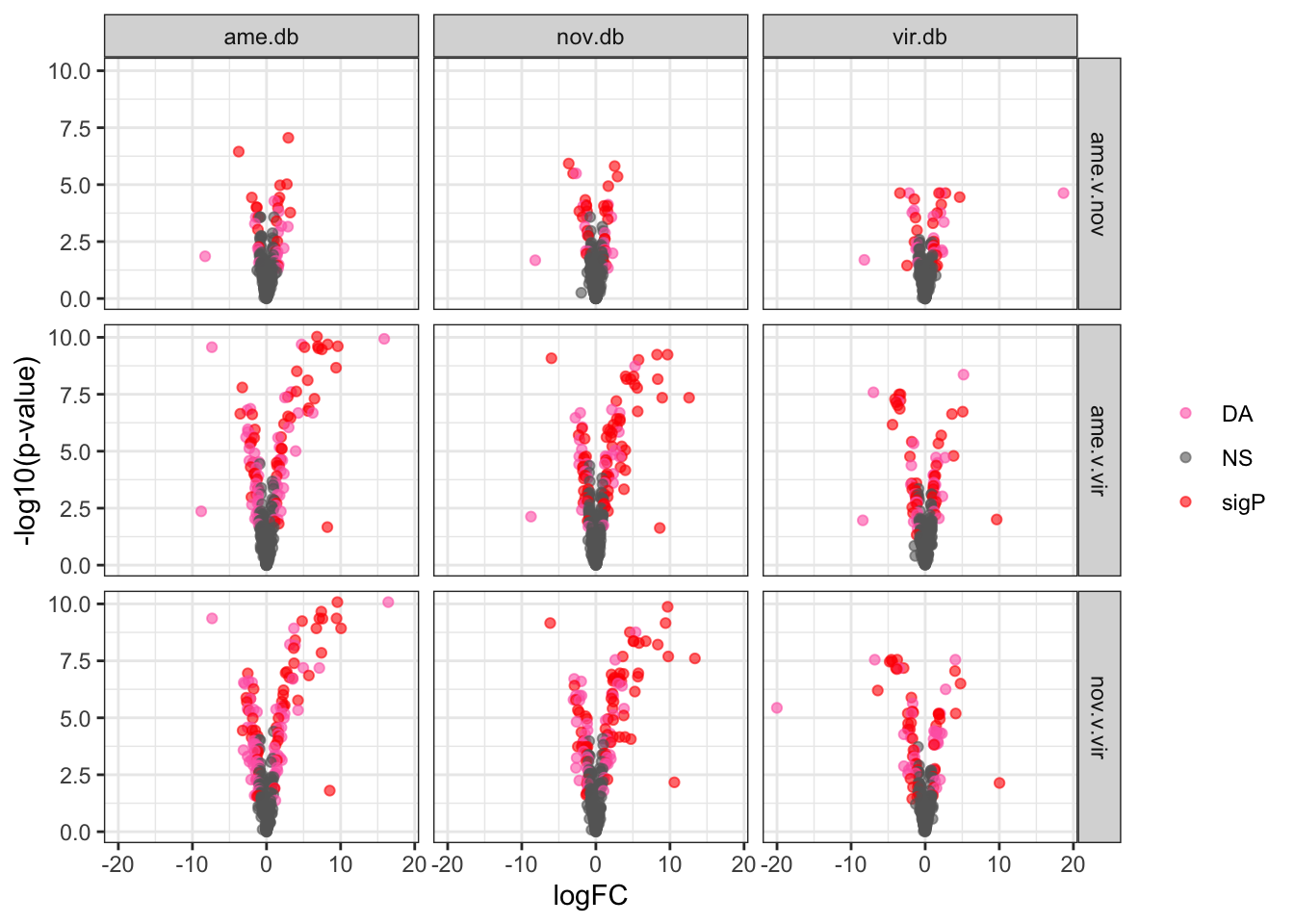
Numbers of differentially abundant proteins more highly abundant in one species vs. the other
bind_rows(ame_MATED,
          nov_MATED,
          vir_MATED) %>% filter(threshold != 'NS') %>%
  mutate(up = ifelse(logFC > 1, 'a', 'b')) %>%
  group_by(comparison, DB, up) %>% dplyr::count() %>%
  ggplot(aes(x = up, y = n, fill = up)) +
  geom_col() +
  facet_grid(comparison ~ DB)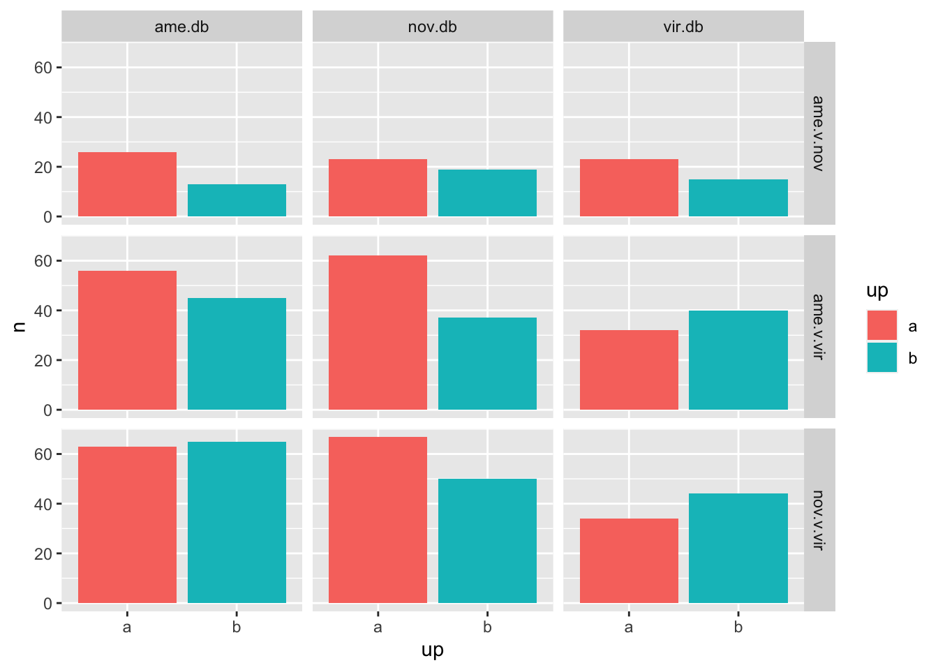
We tested whether signal peptides are more likely to be differentially abundant between species than other proteins
bind_rows(ame_MATED,
          nov_MATED,
          vir_MATED) %>%
  group_by(comparison, DB, threshold, sigP) %>% dplyr::count() %>%
  ggplot(aes(x = sigP, y = n, fill = threshold)) +
  geom_col(position = 'fill') +
  facet_grid(comparison ~ DB)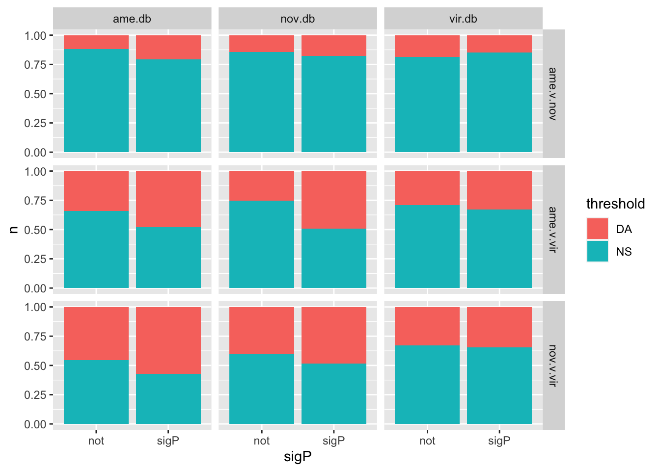
# do Fisher's exact tests
fish_sig <- bind_rows(
  ame_MATED %>%
    group_by(comparison) %>%
    do(fit = broom::tidy(fisher.test(as.matrix(xtabs(~ threshold + sigP, ., sparse = TRUE))))) %>%
    unnest(fit) %>%
    mutate(db = 'ame.db'),
  nov_MATED %>%
    group_by(comparison) %>%
    do(fit = broom::tidy(fisher.test(as.matrix(xtabs(~ threshold + sigP, ., sparse = TRUE))))) %>%
    unnest(fit) %>%
    mutate(db = 'nov.db'),
  vir_MATED %>%
    group_by(comparison) %>%
    do(fit = broom::tidy(fisher.test(as.matrix(xtabs(~ threshold + sigP, ., sparse = TRUE))))) %>%
    unnest(fit) %>%
         mutate(db = 'vir.db'))

fish_sig$FDR <- p.adjust(fish_sig$p.value, method = 'fdr')

fish_sig %>%
  mutate(p.val = ifelse(FDR < 0.001, '< 0.001', round(FDR, 3)),
         comparison = recode(comparison,
                      ame.v.nov = "D. ame vs. D. nov",
                      ame.v.vir = "D. ame vs. D. vir",
                      nov.v.vir = 'D. nov vs. D. vir'),
         across(2:5, ~ round(.x, 2)),
         Estimate = paste0(estimate, ' (', conf.low, '-', conf.high, ')')) %>%
  dplyr::select(Comparison = comparison, Estimate, p.val) %>%
  kable(digits = 3,
        caption = 'Fisher\'s exact tests comparing the representation of signal peptides in differentially abundant proteins between species using each species database. P-values are corrected for multiple testing') %>%
  kable_styling(full_width = FALSE) %>%
  group_rows("D. americana", 1, 3) %>%
  group_rows("D. novamexicana", 4, 6) %>%
group_rows("D. virilis", 7, 9)| Comparison | Estimate | p.val |
|---|---|---|
| D. americana | ||
| D. ame vs. D. nov | 0.51 (0.24-1.07) | 0.161 |
| D. ame vs. D. vir | 0.57 (0.33-0.98) | 0.156 |
| D. nov vs. D. vir | 0.62 (0.36-1.06) | 0.161 |
| D. novamexicana | ||
| D. ame vs. D. nov | 0.78 (0.38-1.59) | 0.64 |
| D. ame vs. D. vir | 0.35 (0.2-0.61) | < 0.001 |
| D. nov vs. D. vir | 0.72 (0.43-1.21) | 0.386 |
| D. virilis | ||
| D. ame vs. D. nov | 1.28 (0.6-2.74) | 0.64 |
| D. ame vs. D. vir | 0.83 (0.45-1.52) | 0.64 |
| D. nov vs. D. vir | 0.93 (0.52-1.67) | 0.889 |
Divergence between (virgin) female reproductive tracts
Here we compare the abundance of proteins in virgin samples between species to investigate divergence in female reproductive tract proteins between species. First we filter out “ejaculate candidates” and only use virgin samples for making comparisons.
# already filtered 2 unique peptides
ame_virgin <- ame_abund %>% filter(!protein %in% ejac_cands$genes[ejac_cands$DB == 'ame.db']) %>%
  dplyr::select(protein, !contains('M'), -UP)
nov_virgin <- nov_abund %>% filter(!protein %in% ejac_cands$genes[ejac_cands$DB == 'nov.db']) %>%
  dplyr::select(protein, !contains('M'), -UP)
vir_virgin <- vir_abund %>% filter(!protein %in% ejac_cands$genes[ejac_cands$DB == 'vir.db']) %>%
  dplyr::select(protein, !contains('M'), -UP)

# get sample info - same for all db's
sampInfo.v = data.frame(condition = str_sub(colnames(ame_virgin[-1]), 1, 2),
                        Replicate = str_sub(colnames(ame_virgin[-1]), 3, 3))

# make design matrix to test diffs between groups
design.v <- model.matrix(~0 + sampInfo.v$condition)
colnames(design.v) <- unique(sampInfo.v$condition)
rownames(design.v) <- sampInfo.v$Replicate

# make contrasts - higher values = higher in mated
cont.virgin <- makeContrasts(a.v.n = AV - NV,
                             a.v.v = AV - VV,
                             n.v.v = NV - VV,
                             levels = design.v)

# create DGElist and fit model
dge_ame.v <- DGEList(counts = ame_virgin[, -1], genes = ame_virgin$protein, group = sampInfo.v$condition)
dge_nov.v <- DGEList(counts = nov_virgin[, -1], genes = nov_virgin$protein, group = sampInfo.v$condition)
dge_vir.v <- DGEList(counts = vir_virgin[, -1], genes = vir_virgin$protein, group = sampInfo.v$condition)

dge_ame.v <- calcNormFactors(dge_ame.v, method = 'TMM')
dge_nov.v <- calcNormFactors(dge_nov.v, method = 'TMM')
dge_vir.v <- calcNormFactors(dge_vir.v, method = 'TMM')

dge_ame.v <- estimateCommonDisp(dge_ame.v)
dge_nov.v <- estimateCommonDisp(dge_nov.v)
dge_vir.v <- estimateCommonDisp(dge_vir.v)

dge_ame.v <- estimateTagwiseDisp(dge_ame.v)
dge_nov.v <- estimateTagwiseDisp(dge_nov.v)
dge_vir.v <- estimateTagwiseDisp(dge_vir.v)

# voom normalisation
dge_ame.v <- voom(dge_ame.v, design.v, plot = FALSE)
dge_nov.v <- voom(dge_nov.v, design.v, plot = FALSE)
dge_vir.v <- voom(dge_vir.v, design.v, plot = FALSE)

# fit linear model
lm_ame.v <- lmFit(dge_ame.v, design = design.v)
lm_nov.v <- lmFit(dge_nov.v, design = design.v)
lm_vir.v <- lmFit(dge_vir.v, design = design.v)

# compare DA between virgin samples

# ame using each database
virgin_an2ame <- contrasts.fit(lm_ame.v, cont.virgin[,"a.v.n"])
virgin_an2nov <- contrasts.fit(lm_nov.v, cont.virgin[,"a.v.n"])
virgin_an2vir <- contrasts.fit(lm_vir.v, cont.virgin[,"a.v.n"])

virgin_an2ame <- eBayes(virgin_an2ame)
virgin_an2nov <- eBayes(virgin_an2nov)
virgin_an2vir <- eBayes(virgin_an2vir)

virgin_an2ame.tTags.table <- topTable(virgin_an2ame, adjust.method = "BH", number = Inf)
virgin_an2nov.tTags.table <- topTable(virgin_an2nov, adjust.method = "BH", number = Inf)
virgin_an2vir.tTags.table <- topTable(virgin_an2vir, adjust.method = "BH", number = Inf)

# nov using each database
virgin_av2ame <- contrasts.fit(lm_ame.v, cont.virgin[,"a.v.v"])
virgin_av2nov <- contrasts.fit(lm_nov.v, cont.virgin[,"a.v.v"])
virgin_av2vir <- contrasts.fit(lm_vir.v, cont.virgin[,"a.v.v"])

virgin_av2ame <- eBayes(virgin_av2ame)
virgin_av2nov <- eBayes(virgin_av2nov)
virgin_av2vir <- eBayes(virgin_av2vir)

virgin_av2ame.tTags.table <- topTable(virgin_av2ame, adjust.method = "BH", number = Inf)
virgin_av2nov.tTags.table <- topTable(virgin_av2nov, adjust.method = "BH", number = Inf)
virgin_av2vir.tTags.table <- topTable(virgin_av2vir, adjust.method = "BH", number = Inf)

# vir using each database
virgin_nv2ame <- contrasts.fit(lm_ame.v, cont.virgin[,"n.v.v"])
virgin_nv2nov <- contrasts.fit(lm_nov.v, cont.virgin[,"n.v.v"])
virgin_nv2vir <- contrasts.fit(lm_vir.v, cont.virgin[,"n.v.v"])

virgin_nv2ame <- eBayes(virgin_nv2ame)
virgin_nv2nov <- eBayes(virgin_nv2nov)
virgin_nv2vir <- eBayes(virgin_nv2vir)

virgin_nv2ame.tTags.table <- topTable(virgin_nv2ame, adjust.method = "BH", number = Inf)
virgin_nv2nov.tTags.table <- topTable(virgin_nv2nov, adjust.method = "BH", number = Inf)
virgin_nv2vir.tTags.table <- topTable(virgin_nv2vir, adjust.method = "BH", number = Inf)

# combine results
ame_VIRGIN <- rbind(virgin_an2ame.tTags.table %>% mutate(comparison = 'ame.v.nov'),
                    virgin_av2ame.tTags.table %>% mutate(comparison = 'ame.v.vir'),
                    virgin_nv2ame.tTags.table %>% mutate(comparison = 'nov.v.vir')) %>%
  mutate(DB = 'ame.db',
         threshold = if_else(adj.P.Val < 0.05 & abs(logFC) > 1, 'DA', 'NS'),
         # add variable for signal peptides reaching significance threshold
         sigP = case_when(genes %in% ame_sig$protein & threshold == 'DA' ~ 'sigP',
                          threshold == 'DA' ~ 'DA',
                          TRUE ~ 'NS'))

nov_VIRGIN <- rbind(virgin_an2nov.tTags.table %>% mutate(comparison = 'ame.v.nov'),
                    virgin_av2nov.tTags.table %>% mutate(comparison = 'ame.v.vir'),
                    virgin_nv2nov.tTags.table %>% mutate(comparison = 'nov.v.vir')) %>%
  mutate(DB = 'nov.db',
         threshold = if_else(adj.P.Val < 0.05 & abs(logFC) > 1, 'DA', 'NS'),
         # add variable for signal peptides reaching significance threshold
         sigP = case_when(genes %in% nov_sig$protein & threshold == 'DA' ~ 'sigP',
                          threshold == 'DA' ~ 'DA',
                          TRUE ~ 'NS'))

vir_VIRGIN <- rbind(virgin_an2vir.tTags.table %>% mutate(comparison = 'ame.v.nov'),
                    virgin_av2vir.tTags.table %>% mutate(comparison = 'ame.v.vir'),
                    virgin_nv2vir.tTags.table %>% mutate(comparison = 'nov.v.vir')) %>%
  mutate(DB = 'vir.db',
         threshold = if_else(adj.P.Val < 0.05 & abs(logFC) > 1, 'DA', 'NS'),
         # add variable for signal peptides reaching significance threshold
         sigP = case_when(genes %in% vir_sig$protein & threshold == 'DA' ~ 'sigP',
                          threshold == 'DA' ~ 'DA',
                          TRUE ~ 'NS'))

# plot all vs. all
bind_rows(ame_VIRGIN,
          nov_VIRGIN,
          vir_VIRGIN) %>%
  ggplot(aes(x = logFC, y = -log10(adj.P.Val), colour = sigP)) +
  geom_point(alpha = .6) +
  scale_colour_manual(values = c('hotpink', 'grey40', 'red')) +
  labs(y = '-log10(p-value)') +
  facet_grid(comparison ~ DB) +
  theme_bw() +
  theme(#legend.position = '',
        legend.title = element_blank(),
        legend.background = element_rect(fill = NA)) +
  NULL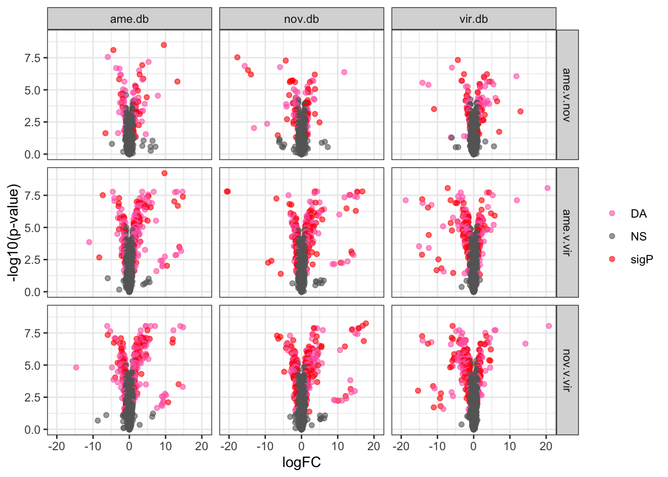
Multi-database analysis
Compiling the species specific database
First we add Orthogroup IDs to proteins identified using each species database. Then we combine the results in to a single dataframe. Finally, we add the list of manually curated ejaculate candidate orthologs which were not assigned to orthogroups. See here for details.
# add orthogroup ID to abundance data
ortho_ame <- tmt_ame_prot %>%
  left_join(orthogroup_long %>% filter(species == 'Dame') %>% select(Orthogroup, protein),
            by = "protein", na_matches = "never") %>%
  rowid_to_column("ID") %>%
  mutate(Orthogroup = if_else(is.na(Orthogroup) == TRUE, paste("AME", ID, sep = "_"),
                              Orthogroup))

ortho_nov <- tmt_nov_prot %>%
  left_join(orthogroup_long %>% filter(species == 'Dnov') %>% select(Orthogroup, protein),
            by = "protein", na_matches = "never") %>%
  rowid_to_column("ID") %>%
  mutate(Orthogroup = if_else(is.na(Orthogroup) == TRUE, paste("NOV", ID, sep = "_"),
                              Orthogroup))

ortho_vir <- tmt_vir_prot %>%
  left_join(orthogroup_long %>% filter(species == 'Dvir') %>% select(Orthogroup, protein),
            by = "protein", na_matches = "never") %>%
  rowid_to_column("ID") %>%
  mutate(Orthogroup = if_else(is.na(Orthogroup) == TRUE, paste("VIR", ID, sep = "_"),
                              Orthogroup))

# total numbers of proteins with orthologs compared to the proteome
bind_cols(N_orth = c(sum(!is.na(orthogroups$Dame)),
                     sum(!is.na(orthogroups$Dnov)),
                     sum(!is.na(orthogroups$Dvir))),
          N_prot = c(11958, 12729, 12792)) %>%
  mutate(prop.orth = N_orth/N_prot)
# A tibble: 3 × 3
N_orth N_prot prop.orth
<int> <dbl> <dbl>
1 8651 11958 0.723
2 9922 12729 0.779
3 9813 12792 0.767# total number of proteins with orthologs in our dataset compared to proteins detected with each database
bind_cols(N_orth = c(n_distinct(ortho_ame %>% filter(str_detect(Orthogroup, "OG")) %>% pull(Orthogroup)),
n_distinct(ortho_nov %>% filter(str_detect(Orthogroup, "OG")) %>% pull(Orthogroup)),
n_distinct(ortho_vir %>% filter(str_detect(Orthogroup, "OG")) %>% pull(Orthogroup))),
N_prot = c(n_distinct(ortho_ame$protein),
n_distinct(ortho_nov$protein),
n_distinct(ortho_vir$protein))) %>%
mutate(prop.orth = N_orth/N_prot)# A tibble: 3 × 3
N_orth N_prot prop.orth
<int> <int> <dbl>
1 2329 3014 0.773
2 2604 3156 0.825
3 2583 3149 0.820# # plot overlap
# upset(fromList(list(
# Dame = na.omit(ortho_ame$Orthogroup),
# Dnov = na.omit(ortho_nov$Orthogroup),
# Dvir = na.omit(ortho_vir$Orthogroup))), order.by = "freq")
plot(euler(c('Dame' = 86, 'Dnov' = 86, 'Dvir' = 90,
'Dame&Dnov' = 98, 'Dame&Dvir' = 73, 'Dnov&Dvir' = 348,
'Dame&Dnov&Dvir' = 2072)),
quantities = TRUE,
fills = list(fill = viridis::viridis(n = 3), alpha = .5))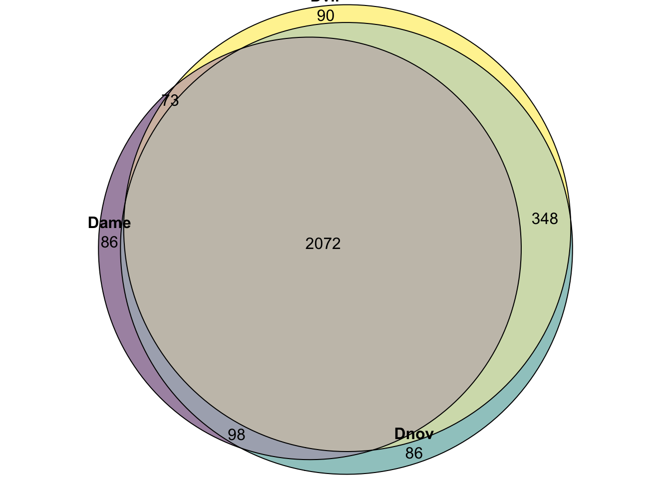
# combine all orthologous data after removing proteins without orthologs
mdb <- ortho_ame %>%
  inner_join(ortho_nov, by = 'Orthogroup', suffix = c('_ame', '_nov'), na_matches = "never") %>%
  inner_join(ortho_vir, by = 'Orthogroup', na_matches = "never") %>%
  relocate(Orthogroup, starts_with("protein"), starts_with("UP")) %>%
  select(-starts_with("ID"))

colnames(mdb)[c(4, 7, 40:55)] <- paste0(colnames(mdb)[c(4, 7, 40:55)], '_vir')

mdb %>% dim
[1] 2621 55mdb %>% map_dbl(n_distinct) Orthogroup protein_ame protein_nov protein_vir UP_ame UP_nov
2072 2160 2145 2141 79 105
UP_vir AM1_ame AM2_ame AM3_ame AV1_ame AV2_ame
103 2160 2159 2159 2160 2159
NM1_ame NM2_ame NM3_ame NV1_ame NV2_ame VM1_ame
2160 2160 2159 2160 2158 2159
VM2_ame VM3_ame VV1_ame VV2_ame VV3_ame AM1_nov
2159 2153 2158 2154 2153 2145
AM2_nov AM3_nov AV1_nov AV2_nov NM1_nov NM2_nov
2143 2144 2143 2144 2145 2144
NM3_nov NV1_nov NV2_nov VM1_nov VM2_nov VM3_nov
2144 2145 2144 2144 2145 2142
VV1_nov VV2_nov VV3_nov AM1_vir AM2_vir AM3_vir
2143 2138 2140 2138 2136 2136
AV1_vir AV2_vir NM1_vir NM2_vir NM3_vir NV1_vir
2138 2138 2137 2138 2137 2141
NV2_vir VM1_vir VM2_vir VM3_vir VV1_vir VV2_vir
2140 2141 2141 2139 2138 2137
VV3_vir
2137 #mdb %>% filter(duplicated(Orthogroup))
#mdb %>% filter(duplicated(protein_ame))
# some proteins are represented more than once due to more than 1:1:1 orthology as they belong to gene families, i.e. orthogroups span multiple genes
#mdb %>% filter(Orthogroup == "OG0000593")
#mdb %>% filter(Orthogroup == "OG0000593") %>% map_dbl(n_distinct)
# which proteins are duplicate members of Orthogroups
# Some proteins are duplicated when merging all databases as they belong to Orthgroups which contain more than one protein. Next we identify proteins which belong to gene families with each database
#ortho_dups <- unique(mdb[which(duplicated(mdb$Orthogroup) == TRUE), "Orthogroup"])
#n_distinct(ortho_dups$Orthogroup)
# # remove proteins with more than 1 to 1 orthology for seperate analysis
# recip_tpp <- mdb %>%
# filter(!Orthogroup %in% ortho_dups$Orthogroup)
# # is equivalent to:
# eqd <- mdb %>%
# filter(!protein_ame %in% mdb$protein_ame[which(duplicated(mdb$protein_ame) == TRUE)],
# !protein_nov %in% mdb$protein_nov[which(duplicated(mdb$protein_nov) == TRUE)],
# !protein_vir %in% mdb$protein_vir[which(duplicated(mdb$protein_vir) == TRUE)])
# dim(recip_tpp)
# colnames(recip_tpp)
#
# recip_tpp %>% map_dbl(n_distinct)
#
# # # write file for dryad
# # write_csv(recip_tpp, 'output/combined_database_tpp.csv')
#
# recip_tpp %>% nrow / tmt_ame_prot %>% nrow()
# recip_tpp %>% nrow / tmt_nov_prot %>% nrow()
# recip_tpp %>% nrow / tmt_vir_prot %>% nrow()
# match the BLAST synteny results between species
a2n_orths <- read.delim("data/orthology_matching/Dame__v__Dnov_blastSyn.txt", header = FALSE) %>%
select(protein_ame = V1, protein_novID = V2) %>%
left_join(read.delim("data/orthology_matching/nov_gene_to_protein.txt", header = FALSE) %>%
select(protein_novID = V1, protein_nov = V2), by = "protein_novID", na_matches = "never") %>%
drop_na(protein_nov)
a2v_orths <- read.delim("data/orthology_matching/Dame__v__Dvir_blastSyn.txt", header = FALSE) %>%
select(protein_ame = V1, protein_virID = V2) %>%
left_join(read.delim("data/orthology_matching/vir_gene_to_protein.txt", header = FALSE) %>%
select(protein_virID = V1, protein_vir = V2), by = "protein_virID", na_matches = "never") %>%
drop_na(protein_vir)
n2a_orths <- read.delim("data/orthology_matching/Dnov__v__Dame_blastSyn.txt", header = FALSE) %>%
select(protein_nov = V1, protein_ameID = V2) %>%
mutate(protein_ame = str_replace(protein_ameID, "\\..\\.p.$", "")) %>%
filter(protein_ame != "")
n2v_orths <- read.delim("data/orthology_matching/Dnov__v__Dvir_blastSyn.txt", header = FALSE) %>%
select(protein_nov = V1, protein_virID = V2) %>%
left_join(read.delim("data/orthology_matching/vir_gene_to_protein.txt", header = FALSE) %>%
select(protein_virID = V1, protein_vir = V2), by = "protein_virID", na_matches = "never") %>%
drop_na(protein_vir)
v2a_orths <- read.delim("data/orthology_matching/Dvir__v__Dame_blastSyn.txt", header = FALSE) %>%
select(protein_vir = V1, protein_ameID = V2) %>%
mutate(protein_ame = str_replace(protein_ameID, "\\..\\.p.$", "")) %>%
filter(protein_ame != "")
v2n_orths <- read.delim("data/orthology_matching/Dvir__v__Dnov_blastSyn.txt", header = FALSE) %>%
select(protein_vir = V1, protein_novID = V2) %>%
left_join(read.delim("data/orthology_matching/nov_gene_to_protein.txt", header = FALSE) %>%
select(protein_novID = V1, protein_nov = V2), by = "protein_novID", na_matches = "never") %>%
drop_na(protein_nov)
# now stick the new nov ID on to the americana data, new ame on to virilis, etc.
sticky_an <- ortho_ame %>% rename(protein_ame = protein) %>%
left_join(a2n_orths, by = "protein_ame", na_matches = "never") %>% drop_na(protein_nov) %>%
left_join(ortho_nov, by = c("protein_nov" = "protein"), suffix = c('_ame', '_nov'), na_matches = "never")
sticky_av <- ortho_ame %>% rename(protein_ame = protein) %>%
left_join(a2v_orths, by = "protein_ame", na_matches = "never") %>% drop_na(protein_vir) %>%
left_join(ortho_vir, by = c("protein_vir" = "protein"), suffix = c('_ame', '_vir'), na_matches = "never")
sticky_na <- ortho_nov %>% rename(protein_nov = protein) %>%
left_join(n2a_orths, by = "protein_nov", na_matches = "never") %>% drop_na(protein_ame) %>%
left_join(ortho_ame, by = c("protein_ame" = "protein"), suffix = c('_nov', '_ame'), na_matches = "never")
sticky_nv <- ortho_nov %>% rename(protein_nov = protein) %>%
left_join(n2v_orths, by = "protein_nov", na_matches = "never") %>% drop_na(protein_vir) %>%
left_join(ortho_vir, by = c("protein_vir" = "protein"), suffix = c('_nov', '_vir'), na_matches = "never")
sticky_va <- ortho_vir %>% rename(protein_vir = protein) %>%
left_join(v2a_orths, by = "protein_vir", na_matches = "never") %>% drop_na(protein_ame) %>%
left_join(ortho_ame, by = c("protein_ame" = "protein"), suffix = c('_vir', '_ame'), na_matches = "never")
sticky_vn <- ortho_vir %>% rename(protein_vir = protein) %>%
left_join(v2n_orths, by = "protein_vir", na_matches = "never") %>% drop_na(protein_nov) %>%
left_join(ortho_nov, by = c("protein_nov" = "protein"), suffix = c('_vir', '_nov'), na_matches = "never")
# combine all the results and merge missing values across rows using 'fill'
ortho_dat <- bind_rows(sticky_an, sticky_av,
sticky_na, sticky_nv,
sticky_va, sticky_vn) %>%
relocate(starts_with("Orthogroup"), starts_with("protein"), starts_with("UP")) %>%
select(-contains("ID")) %>%
group_by(protein_ame) %>%
fill(everything(), .direction = "downup") %>%
slice(1) %>%
group_by(protein_nov) %>%
fill(everything(), .direction = "downup") %>%
slice(1) %>%
group_by(protein_vir) %>%
fill(everything(), .direction = "downup") %>%
slice(1)
# combine orthogroup IDs where possible or make a new ID
ortho_dat <- ortho_dat %>%
bind_cols(Orthogroup = coalesce(coalesce(ortho_dat$Orthogroup_ame,
ortho_dat$Orthogroup_nov), ortho_dat$Orthogroup_vir)) %>%
rowid_to_column("ID") %>%
mutate(Orthogroup = if_else(grepl("OG", Orthogroup) == FALSE, paste("NEWG", ID, sep = "_"),
Orthogroup))
dim(ortho_dat)[1] 63 59ortho_dat %>% map_dbl(n_distinct) ID Orthogroup_ame Orthogroup_nov Orthogroup_vir protein_ame
63 58 48 33 63
protein_nov protein_vir UP_ame UP_nov UP_vir
63 63 20 22 19
AM1_ame AM2_ame AM3_ame AV1_ame AV2_ame
58 58 58 58 58
NM1_ame NM2_ame NM3_ame NV1_ame NV2_ame
58 58 58 58 58
VM1_ame VM2_ame VM3_ame VV1_ame VV2_ame
58 58 58 58 58
VV3_ame AM1_nov AM2_nov AM3_nov AV1_nov
56 48 48 48 48
AV2_nov NM1_nov NM2_nov NM3_nov NV1_nov
48 48 48 48 48
NV2_nov VM1_nov VM2_nov VM3_nov VV1_nov
48 48 48 48 47
VV2_nov VV3_nov AM1_vir AM2_vir AM3_vir
47 47 33 33 33
AV1_vir AV2_vir NM1_vir NM2_vir NM3_vir
33 33 33 33 33
NV1_vir NV2_vir VM1_vir VM2_vir VM3_vir
33 33 33 33 33
VV1_vir VV2_vir VV3_vir Orthogroup
33 33 33 63 # add the new data with the combined database
mdb2 <- bind_rows(mdb, ortho_dat %>% select(-starts_with("Orthogroup_"), -ID))
dim(mdb2)[1] 2684 55mdb2 %>% map_dbl(n_distinct) Orthogroup protein_ame protein_nov protein_vir UP_ame UP_nov
2132 2221 2197 2195 80 106
UP_vir AM1_ame AM2_ame AM3_ame AV1_ame AV2_ame
105 2215 2214 2214 2215 2214
NM1_ame NM2_ame NM3_ame NV1_ame NV2_ame VM1_ame
2215 2215 2214 2215 2213 2213
VM2_ame VM3_ame VV1_ame VV2_ame VV3_ame AM1_nov
2213 2207 2212 2208 2206 2181
AM2_nov AM3_nov AV1_nov AV2_nov NM1_nov NM2_nov
2179 2180 2179 2180 2181 2180
NM3_nov NV1_nov NV2_nov VM1_nov VM2_nov VM3_nov
2180 2181 2180 2180 2181 2178
VV1_nov VV2_nov VV3_nov AM1_vir AM2_vir AM3_vir
2177 2173 2175 2161 2159 2159
AV1_vir AV2_vir NM1_vir NM2_vir NM3_vir NV1_vir
2161 2161 2160 2161 2160 2164
NV2_vir VM1_vir VM2_vir VM3_vir VV1_vir VV2_vir
2163 2164 2164 2162 2161 2160
VV3_vir
2160 # proportion of each database represented by Orthogrous in the combined database
n_distinct(mdb2$Orthogroup) / c(n_distinct(ortho_ame$protein),
n_distinct(ortho_nov$protein),
n_distinct(ortho_vir$protein))[1] 0.7073656 0.6755387 0.6770403# duplicated orthogroups
ortho_dups <- mdb2 %>%
filter(Orthogroup %in% unique(mdb2[which(duplicated(mdb2$Orthogroup) == TRUE), "Orthogroup"])$Orthogroup)
dim(ortho_dups)[1] 669 55n_distinct(ortho_dups$Orthogroup)[1] 117# number of single copy orthogroups
mdb2 %>% filter(!Orthogroup %in% ortho_dups$Orthogroup) %>% dim()[1] 2015 55mdb2 %>% filter(Orthogroup %in% ortho_dups$Orthogroup) %>% dim()[1] 669 55# count the numbers of proteins and numbers of proteins belonging to each orthogroup
mdb_counts <- mdb2 %>%
group_by(Orthogroup) %>%
summarise(ame = n_distinct(protein_ame),
nov = n_distinct(protein_nov),
vir = n_distinct(protein_vir)) %>%
pivot_longer(cols = 2:4)
# number of proteins belonging to an orthogroup - most proteins are single copy
mdb_counts %>%
group_by(name, value) %>%
count() %>%
mutate(N2 = ifelse(value > 6, "7+", as.character(value)),
n2 = ifelse(value == 1, n/10, n)) %>%
#ggplot(aes(x = N2, y = n2, fill = species)) +
ggplot(aes(x = value, y = n2, fill = name)) +
geom_bar(stat = "identity", position = "dodge") +
scale_fill_viridis_d(name = "Species: ",
labels = c(expression(italic('D. ame')),
expression(italic('D. nov')),
expression(italic('D. vir')))) +
labs(x = "Copy number", y = "Count") +
theme_bw() +
theme(legend.position = "bottom") +
#ggsave('plots/TPP_results/orthogroup_counts.pdf', height = 4, width = 4, dpi = 600, useDingbats = FALSE) +
NULL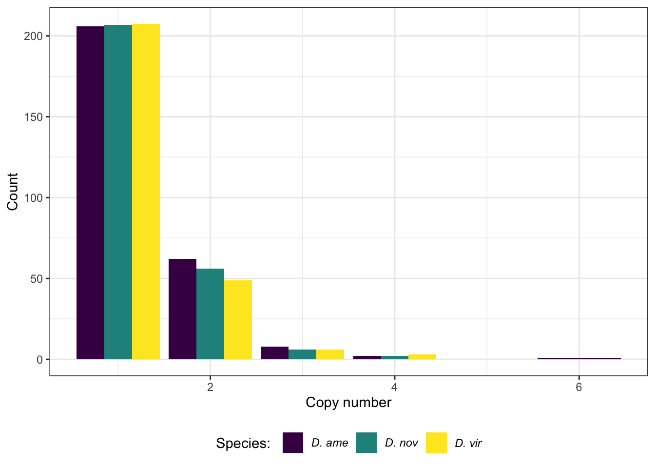
sco_mdb <- mdb_counts %>%
  group_by(Orthogroup, value) %>%
  count(name = "N") %>% filter(N == 3)

mdb_counts %>%
  #filter(!Orthogroup %in% sco_mdb$Orthogroup) %>%
  filter(Orthogroup %in% ortho_dups$Orthogroup) %>%
  group_by(Orthogroup, name, value) %>%
  count(name = "N") %>% ungroup() %>%
  mutate(value = factor(value)) %>%
  ggplot(aes(x = name, stratum = value, alluvium = Orthogroup,
             y = N, label = value)) +
  #geom_flow(aes(fill = value)) +
  geom_alluvium(aes(fill = value)) +
  geom_stratum(aes(fill = value)) +
  geom_text(stat = "stratum") +
  scale_fill_viridis_d(name = "Copy no.") +
  labs(x = "Species", y = "No. proteins") +
  theme_bw() +
  #ggsave('plots/TPP_results/alluvial_duplicates.pdf', height = 6.4, width = 4.8, dpi = 600, useDingbats = FALSE) +
  NULL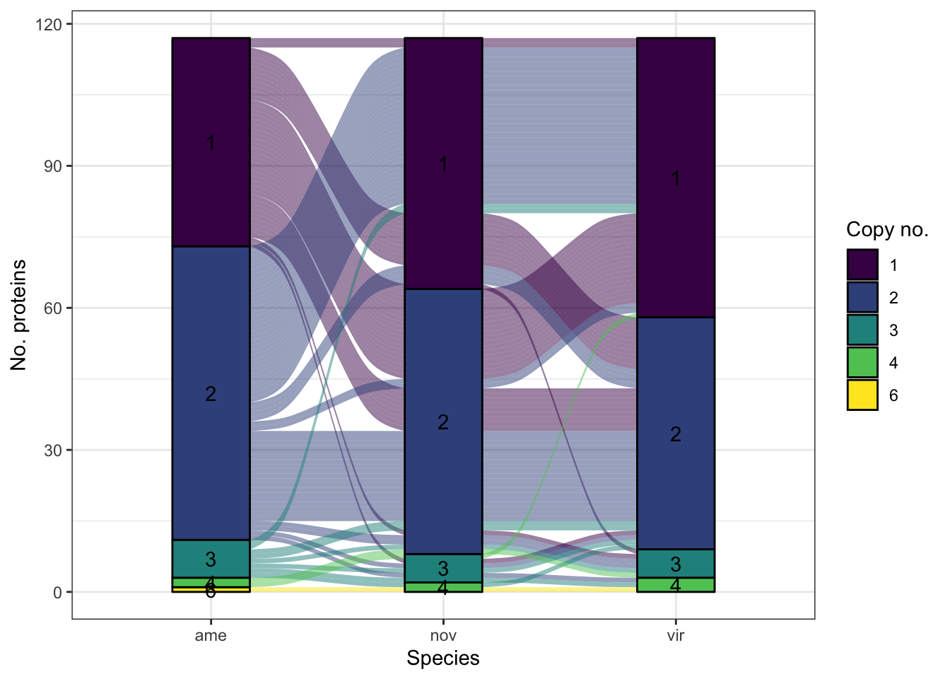
# ortho_dups %>%
#   group_by(Orthogroup) %>%
#   mutate(unique_ame = n_distinct(protein_ame),
#          unique_nov = n_distinct(protein_nov),
#          unique_vir = n_distinct(protein_vir)) %>%
#   #select(Orthogroup, starts_with("unique")) %>%
#   distinct(Orthogroup, unique_ame, unique_nov, unique_vir) %>%
#   pivot_longer(cols = 2:4) %>%
#   ggplot(aes(x = name, y = Orthogroup, fill = value)) +
#   geom_tile() +
#   scale_fill_viridis_c()
Differential abundance analysis
We performed differential abundance analyses using the combined database with species-specific abundance data collated using each iterative run from the TPP.
# filter must have two unique peptides in at least 1 dataset
multiDB <- mdb2 %>%
  filter(UP_ame >= 2 | UP_nov >= 2 | UP_vir >= 2) %>%
  dplyr::select(protein_vir, Orthogroup,
                AM1_ame, AM2_ame, AM3_ame, AV1_ame, AV2_ame,
                NM1_nov, NM2_nov, NM3_nov, NV1_nov, NV2_nov,
                VM1_vir, VM2_vir, VM3_vir, VV1_vir, VV2_vir, VV3_vir) %>%
  mutate(across(3:18, ~replace_na(.x, 0)))

colnames(multiDB)[3:18] <- gsub('_.*', '', x = colnames(multiDB)[3:18])

# make object for protein abundance data and replace NA's with 0's
expr_data <- multiDB[, -c(1:2)]

# get sample info
sampInfo = data.frame(species = str_sub(colnames(expr_data), 1, 1),
                      mating = str_sub(colnames(expr_data), 2, 2),
                      condition = str_sub(colnames(expr_data), 1, 2),
                      Replicate = str_sub(colnames(expr_data), -1))

# make design matrix to test diffs between groups
design <- model.matrix(~0 + sampInfo$condition)
colnames(design) <- unique(sampInfo$condition)
rownames(design) <- sampInfo$Replicate

# create DGElist and fit model
dgeList <- DGEList(counts = expr_data, genes = multiDB$protein_vir, group = sampInfo$condition)
dgeList <- calcNormFactors(dgeList, method = 'TMM')
dgeList <- estimateCommonDisp(dgeList)
dgeList <- estimateTagwiseDisp(dgeList)

# make contrasts - higher values = higher in mated
cont.matrix <- makeContrasts(M.a.V = AM - AV,
                             M.n.V = NM - NV,
                             M.v.V = VM - VV,
                             levels = design)

# voom normalisation
dgeListV <- voom(dgeList, design, plot = FALSE)

# fit linear model
lm_fit <- lmFit(dgeListV, design = design)
Heatmap
All replicates
# make DF
sample_voomed <- data.frame(genes = dgeListV$genes,
                            dgeListV$E) %>%
  left_join(vir_fbgn %>% select(-FBtr), by = c('genes' = 'gene_id'), na_matches = "never") %>%
  # add mel Sfp ortholog
  left_join(wigbySFP %>% dplyr::select(FBgn, mel_Sfp = Symbol), na_matches = "never") %>%
  # add annotations
  mutate(Ejac = ifelse(genes %in% vir_cands$genes, 'Ejac', NA),
         sperm = ifelse(FBgn %in% sperm_mel$FBgn_v, 'sperm', NA),
         sigP = ifelse(genes %in% vir_sig$protein, 'sig', NA),
         #mel_Sfp = ifelse(FBgn %in% wigbySFP$FBgn, 'Sfp', NA),
         category = case_when(FBgn %in% sperm_mel$FBgn_v ~ 'sperm',
                              FBgn %in% wigbySFP$FBgn ~ 'Sfp',
                              genes %in% vir_sig$protein ~ 'sigP',
                              TRUE ~ 'other')) %>%
  distinct(genes, Orthogroup, .keep_all = TRUE) %>%
  mutate(dupl = ifelse(Orthogroup %in% ortho_dups$Orthogroup, "Dup", "not"))

samp_vm <- sample_voomed %>% dplyr::select(genes, FBgn, 2:17, mel_Sfp, category)

#row.names(samp_vm) <- sample_voomed$genes

vm_scaled <- as.matrix(pheatmap:::scale_rows(sample_voomed[, 2:17]))
colnames(vm_scaled) <- colnames(sample_voomed[, 2:17])

# heatmap annotations
labs1 <- rowAnnotation(cat_lab = sample_voomed$category,
                       col = list(cat_lab = c(sperm = v.pal[2],
                                              Sfp = v.pal[3],
                                              sigP = v.pal[1],
                                              other = NA)),
                       Sfp_labs = anno_mark(at = c(grep('Sfp', x = sample_voomed$category)),
                                            labels = sample_voomed$mel_Sfp[sample_voomed$category == 'Sfp'],
                                            labels_gp = gpar(fontsize = 5)),
                       title = NULL,
                       show_annotation_name = FALSE)

dupl_lab <- rowAnnotation(Dupl = sample_voomed$dupl,
                          col = list(Dupl = c(Dup = "red", not = NA)),
                          title = NULL,
                          show_annotation_name = FALSE)

vmha <- HeatmapAnnotation(species = str_sub(colnames(samp_vm[, 3:18]), 1, 1),
                          mating = str_sub(colnames(samp_vm[, 3:18]), 2, 2),
                          col = list(species = c('V' = v.pal[1],
                                                 'N' = v.pal[2],
                                                 'A' = v.pal[3]),
                                     mating = c('M' = viridis::magma(n = 4)[3],
                                                'V' = viridis::magma(n = 4)[2])))

#pdf('plots/TPP_results/TPP_all_compheatmap.pdf', height = 8, width = 5)
Heatmap(vm_scaled,
        #col = viridis::inferno(100),
        heatmap_legend_param = list(title = "log2(intensities)",
                                    title_position = "leftcenter-rot"),
        left_annotation = dupl_lab,
        right_annotation = labs1,
        top_annotation = vmha,
        show_row_names = FALSE,
        show_column_names = FALSE,
        column_split = 3,
        column_gap = unit(0, "mm"),
        row_title = NULL,
        column_title = NULL)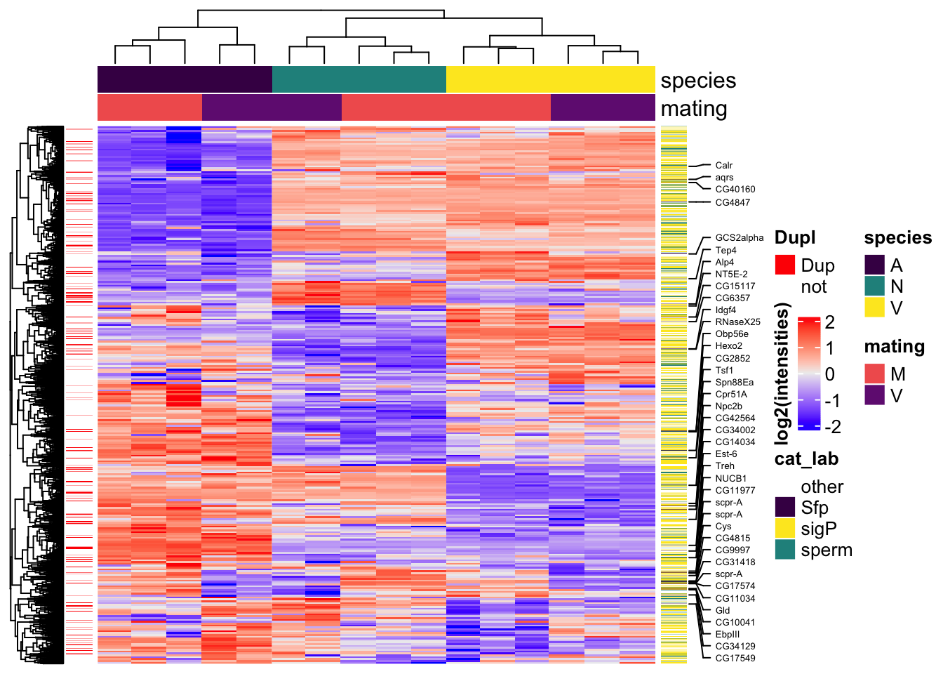
#dev.off()Sample medians
# make DF
sample_medians <- data.frame(genes = dgeListV$genes,
                             dgeListV$E) %>%
  rowwise() %>%
  mutate(AM = median(c(!!! rlang::syms(grep('AM', names(.), value = TRUE)))),
         NM = median(c(!!! rlang::syms(grep('NM', names(.), value = TRUE)))),
         VM = median(c(!!! rlang::syms(grep('VM', names(.), value = TRUE)))),
         AV = median(c(!!! rlang::syms(grep('AV', names(.), value = TRUE)))),
         NV = median(c(!!! rlang::syms(grep('NV', names(.), value = TRUE)))),
         VV = median(c(!!! rlang::syms(grep('VV', names(.), value = TRUE))))) %>%
  dplyr::select(genes, AM, NM, VM, AV, NV, VV) %>%
  left_join(vir_fbgn %>% select(-FBtr), by = c('genes' = 'gene_id')) %>%
  # add mel Sfp ortholog
  left_join(wigbySFP %>% dplyr::select(FBgn, mel_Sfp = Symbol)) %>%
  # add annotations
  mutate(Ejac = ifelse(genes %in% vir_cands$genes, 'Ejac', NA),
         sperm = ifelse(FBgn %in% sperm_mel$FBgn_v, 'sperm', NA),
         sigP = ifelse(genes %in% vir_sig$protein, 'sig', NA),
         #mel_Sfp = ifelse(FBgn %in% wigbySFP$FBgn, 'Sfp', NA),
         category = case_when(FBgn %in% sperm_mel$FBgn_v ~ 'sperm',
                              FBgn %in% wigbySFP$FBgn ~ 'Sfp',
                              genes %in% vir_sig$protein ~ 'sigP',
                              TRUE ~ 'other')) %>%
  distinct(genes, Orthogroup, .keep_all = TRUE)

samp_hm <- sample_medians %>% dplyr::select(genes, FBgn, 2:7, mel_Sfp, category)

#row.names(samp_hm) <- sample_medians$genes

mat_scaled <- as.matrix(pheatmap:::scale_rows(sample_medians[, 2:7]))
colnames(mat_scaled) <- colnames(sample_medians[, 2:7])

labs2 <- rowAnnotation(cat_lab = sample_medians$category,
                       col = list(cat_lab = c(sperm = v.pal[2],
                                              Sfp = v.pal[3],
                                              sigP = v.pal[1],
                                              other = NA)),
                       Sfp_labs = anno_mark(at = c(grep('Sfp', x = sample_medians$category)),
                                            labels = sample_medians$mel_Sfp[sample_medians$category == 'Sfp'],
                                            labels_gp = gpar(fontsize = 5)),
                       title = NULL,
                       show_annotation_name = FALSE)

mdha <- HeatmapAnnotation(species = str_sub(colnames(samp_hm[, 3:8]), 1, 1),
                          mating = str_sub(colnames(samp_hm[, 3:8]), 2, 2),
                          col = list(species = c('V' = v.pal[1],
                                                 'N' = v.pal[2],
                                                 'A' = v.pal[3]),
                                     mating = c('M' = viridis::magma(n = 4)[3],
                                                'V' = viridis::magma(n = 4)[2])))

#pdf('plots/TPP_results/TPP_all_hm-md.pdf', height = 8, width = 5)
Heatmap(mat_scaled,
        col = viridis::inferno(50),
        heatmap_legend_param = list(title = "log2(intensities)",
                                    title_position = "leftcenter-rot"),
        right_annotation = labs2,
        top_annotation = mdha,
        show_row_names = FALSE,
        show_column_names = FALSE,
        column_split = 3,
        column_gap = unit(0, "mm"),
        row_title = NULL,
        column_title = NULL)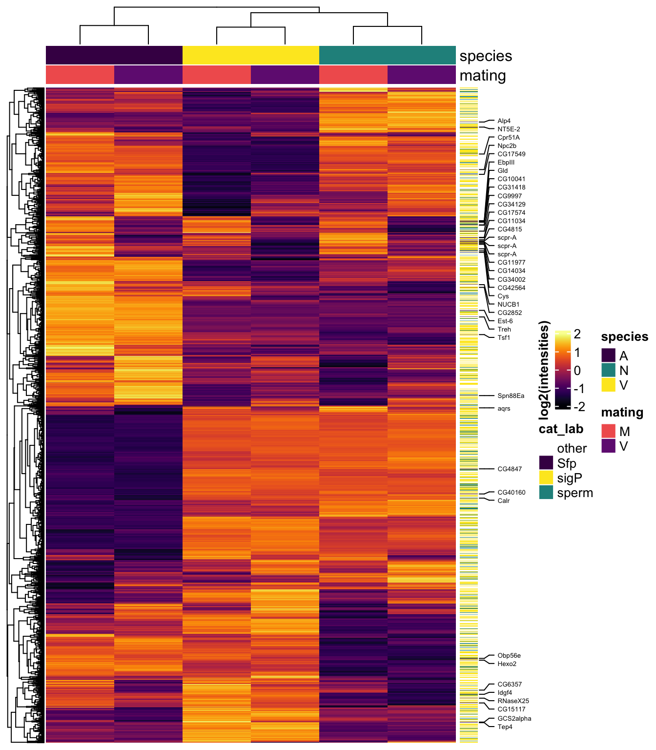
#dev.off()Diagnostic plots
par(mfrow = c(2,2))
# Biological coefficient of variation
plotBCV(dgeList)
# mean-variance trend
voomed = voom(dgeList, design, plot = TRUE)
# QQ-plot
g <- gof(glmFit(dgeList, design))
z <- zscoreGamma(g$gof.statistics,shape = g$df/2,scale = 2)
qqnorm(z); qqline(z, col = 4,lwd = 1, lty = 1)
# log2 transformed and normalize boxplot of counts across samples
boxplot(voomed$E, xlab = "", ylab = "log2(Abundance)", las = 2 , main = "Voom transformed logCPM",
        col = c(rep(brewer.pal(n = 6, name = 'Spectral'), each = 3)[-c(6,12)]))
abline(h = median(voomed$E), col = "blue")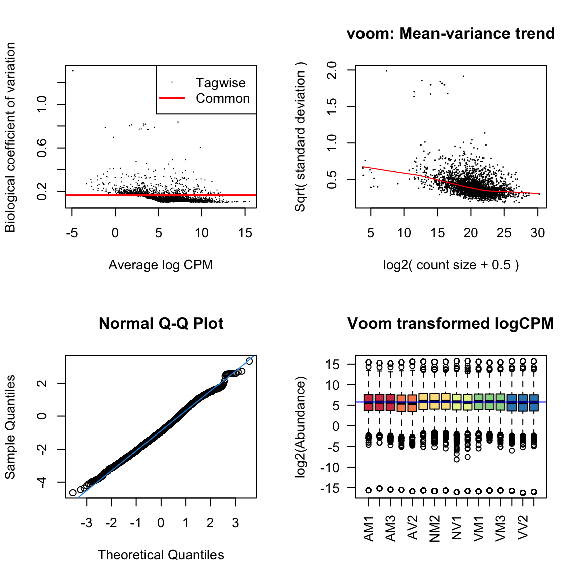
par(mfrow = c(1,1))Principal component analysis
# pca <- prcomp(t(dgeListV$E %>% as_tibble()), center = TRUE, scale. = TRUE)
# # broom::tidy(pca, 'pcs') %>%
# #   mutate(percent = percent * 100,
# #          cumulative = cumulative * 100)
#
# PCA_dat <- as.data.frame(pca$x)[, 1:3] %>%
#   rownames_to_column() %>%
#   mutate(species = str_sub(rowname, 1, 1),
#          mating = str_sub(rowname, 2, 2),
#          condition = str_sub(rowname, 1, 2))

# only most variable proteins
most_var <- dgeListV$E %>% as_tibble() %>%
  # exclude duplicated orthogroups
  slice(-which(duplicated(multiDB$Orthogroup) == TRUE)) %>%
  mutate(vars = apply(., 1, var)) %>%
  slice_max(vars, n = 500) %>%
  select(-vars)

pca.mostvar <- prcomp(t(as.matrix(most_var)), center = TRUE, scale. = TRUE)
# broom::tidy(pca.mostvar, 'pcs') %>%
#   mutate(percent = percent * 100,
#          cumulative = cumulative * 100)

PCA_mostvar <- as.data.frame(pca.mostvar$x)[, 1:3] %>%
  rownames_to_column() %>%
  mutate(species = str_sub(rowname, 1, 1),
         mating = str_sub(rowname, 2, 2),
         condition = str_sub(rowname, 1, 2))

# # Plot for figure
# PCA_mostvar %>%
#   ggplot(aes(x = PC1, y = PC2, colour = species, shape = mating)) +
#   geom_point(size = 8, alpha = .7) +
#   labs(x = paste0('PC1 (', (100*round(summary(pca.mostvar)$importance[2, 1], 3)), '%)'),
#        y = paste0('PC2 (', (100*round(summary(pca.mostvar)$importance[2, 2], 3)), '%)')) +
#   scale_colour_viridis_d(labels = c(expression(italic('D. ame')),
#                                     expression(italic('D. nov')),
#                                     expression(italic('D. vir')))) +
#   scale_shape_manual(values = c(16, 18), labels = c('Mated', 'Virgin')) +
#   theme_bw() +
#   theme(legend.title = element_blank(),
#         legend.text.align = 0,
#         legend.text = element_text(size = 12),
#         legend.background = element_blank(),
#         axis.text = element_text(size = 10),
#         axis.title = element_text(size = 12)) +
#   #ggsave('plots/TPP_results/TPP_PCA_12.pdf', height = 3.4, width = 4.8, dpi = 600, useDingbats = FALSE) +
#   NULL

rbind(as.matrix(PCA_mostvar[, c(2, 3)]),
      as.matrix(PCA_mostvar[, c(2, 4)]),
      as.matrix(PCA_mostvar[, c(3, 4)])) %>%
  bind_cols(species = rep(PCA_mostvar$species, 3),
            mating = rep(PCA_mostvar$mating, 3),
            pc = rep(c(paste0('PC1 (',100*round(summary(pca.mostvar)$importance[2, 1], 3), '%) vs. PC2 (',
                              100*round(summary(pca.mostvar)$importance[2, 2], 3), '%)'),
                       paste0('PC1 (',100*round(summary(pca.mostvar)$importance[2, 1], 3), '%) vs. PC3 (',
                              100*round(summary(pca.mostvar)$importance[2, 3], 3), '%)'),
                       paste0('PC2 (',100*round(summary(pca.mostvar)$importance[2, 2], 3), '%) vs. PC3 (',
                              100*round(summary(pca.mostvar)$importance[2, 3], 3), '%)')),
                     each = 16)) %>%
  ggplot(aes(x = PC1, y = PC2, colour = species, shape = mating, alpha = .5)) +
  geom_point(size = 8, alpha = .7) +
  scale_colour_viridis_d(labels = c(expression(italic('D. ame')),
                                    expression(italic('D. nov')),
                                    expression(italic('D. vir')))) +
  scale_shape_manual(values = c(16, 18), labels = c('Mated', 'Virgin')) +
  facet_wrap(~pc) +
  theme_bw() +
  theme(legend.title = element_blank(),
        legend.text.align = 0,
        legend.text = element_text(size = 12),
        legend.background = element_blank(),
        axis.text = element_text(size = 10),
        axis.title = element_blank(),
        strip.text = element_text(size = 15)) +
  NULL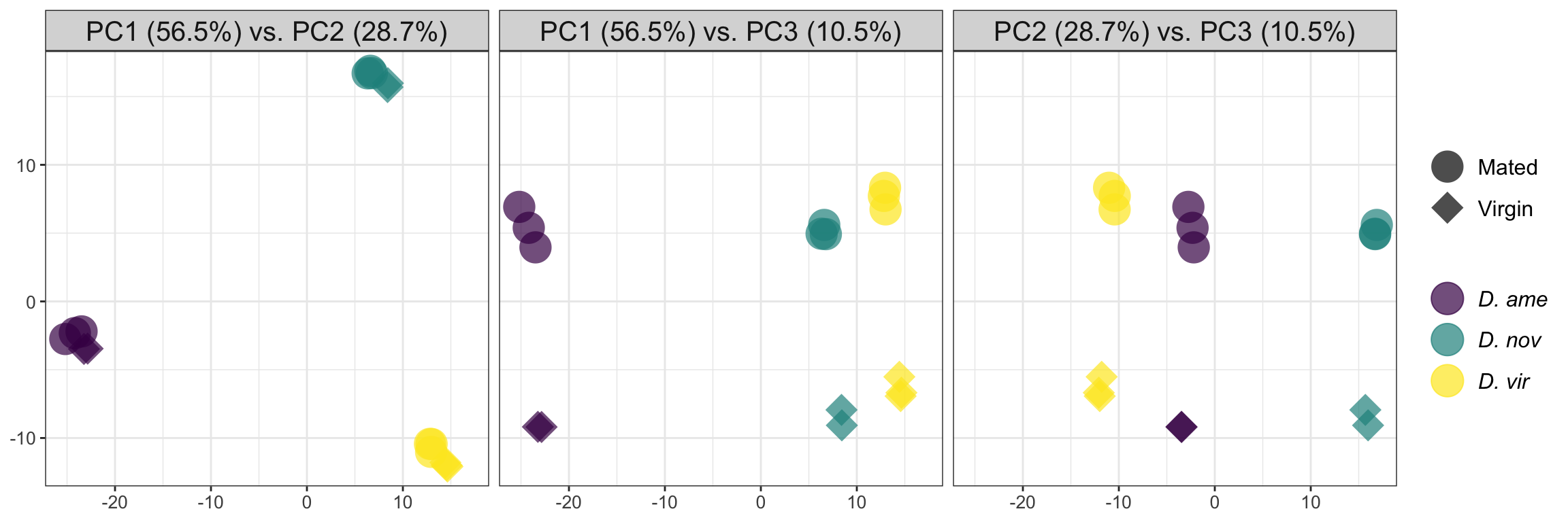
Identifying ejaculate candidates
We compared abundances between mated and virgin samples for each species.
# perform lmFit tests
# ame
lm_ame <- contrasts.fit(lm_fit, cont.matrix[,"M.a.V"])
lm_ame <- eBayes(lm_ame)
lm_ame.tTags.table <- topTable(lm_ame, adjust.method = "BH", number = Inf) %>%
  mutate(species = "ame",
         threshold = if_else(adj.P.Val < 0.05 & abs(logFC) > 1, "SD", "NS"))

# nov
lm_nov <- contrasts.fit(lm_fit, cont.matrix[,"M.n.V"])
lm_nov <- eBayes(lm_nov)
lm_nov.tTags.table <- topTable(lm_nov, adjust.method = "BH", number = Inf) %>%
  mutate(species = "nov",
         threshold = if_else(adj.P.Val < 0.05 & abs(logFC) > 1, "SD", "NS"))

# vir
lm_vir <- contrasts.fit(lm_fit, cont.matrix[,"M.v.V"])
lm_vir <- eBayes(lm_vir)
lm_vir.tTags.table <- topTable(lm_vir, adjust.method = "BH", number = Inf) %>%
  mutate(species = "vir",
         threshold = if_else(adj.P.Val < 0.05 & abs(logFC) > 1, "SD", "NS"))

comb_TABLES <- rbind(lm_ame.tTags.table,
                     lm_nov.tTags.table,
                     lm_vir.tTags.table) %>%
  left_join(vir_fbgn %>% select(-FBtr), by = c('genes' = 'gene_id'), na_matches = "never") %>%
  mutate(
    # add variable for signal peptides reaching significance threshold
    sigP = if_else(genes %in% vir_sig$protein, 'sigP', 'not'),
    # add variable splitting by bias to virgin vs. mated and signal peptide
    sperm = if_else(FBgn %in% sperm_mel$FBgn_v, 'Sperm', 'not'),
    # add variable splitting by bias to virgin vs. mated and signal peptide
    DA = case_when(threshold == 'SD' & logFC > 1 & sigP == 'sigP' ~ "MBsec",
                   threshold == 'SD' & logFC < -1 & sigP == 'sigP' ~ "FMsec",
                   threshold == 'SD' & logFC > 1 ~ "MB",
                   threshold == 'SD' & logFC < -1 ~ "FM",
                   TRUE ~ 'NS')) %>%
  distinct(genes, species, .keep_all = TRUE)

# remove duplicated genes
comb_TABLES_nd <- comb_TABLES %>% filter(!Orthogroup %in% ortho_dups$Orthogroup)

# save differentially abundant proteins to table for ClueGO
ejac_cands_multiDB <- comb_TABLES %>% filter(adj.P.Val < 0.05 & logFC > 1) %>%
  distinct(genes, .keep_all = TRUE)

#ejac_cands_multiDB %>% map_dbl(n_distinct)

# ejac_cands_multiDB %>% write_csv('output/ClueGOlists/TPP_ejac_cands_multiDB_mel.csv')

# number of Dmel Sperm proteins id'd
ejac_cands_multiDB %>%
  left_join(sperm_mel, by = c("FBgn" = "FBgn_v")) %>%
  distinct(FBgn, .keep_all = TRUE) %>% drop_na(mel_FBgn_ID) %>%
  select(FBgn, mel_FBgn_ID, Gene.Symbol) %>%
  kable(caption = 'D. melanogaster sperm protein orthologs') %>%
kable_styling(full_width = FALSE)| FBgn | mel_FBgn_ID | Gene.Symbol |
|---|---|---|
| FBgn0210936 | FBgn0038395 | CG10407 |
| FBgn0203892 | FBgn0086907 | Cyt-c-d |
| FBgn0210972 | FBgn0051872 | CG31872 |
| FBgn0204803 | FBgn0260453 | CG17140 |
| FBgn0211422 | FBgn0039257 | tnc |
| FBgn0205934 | FBgn0031171 | CG1801 |
| FBgn0204735 | FBgn0031869 | CG18304 |
| FBgn0205696 | FBgn0030362 | regucalcin |
| FBgn0198514 | FBgn0015278 | Pi3K68D |
| FBgn0197452 | FBgn0013812 | Dhc93AB |
| FBgn0202027 | FBgn0030482 | CG1673 |
| FBgn0203308 | FBgn0027560 | Tps1 |
| FBgn0201010 | FBgn0266136 | Gyc76C |
| FBgn0199271 | FBgn0051644 | CG31644 |
| FBgn0199705 | FBgn0046704 | Liprin-alpha |
| FBgn0204802 | FBgn0069354 | Porin2 |
| FBgn0210522 | FBgn0037891 | CG5214 |
| FBgn0204328 | FBgn0004507 | GlyP |
| FBgn0202308 | FBgn0001187 | Hex-C |
| FBgn0016474 | FBgn0004045 | Yp1 |
# number of Dmel SFPs id'd
ejac_cands_multiDB %>% left_join(wigbySFP, by = "FBgn") %>% drop_na(FBgn_mel) %>%
  distinct(FBgn, FBgn_mel, Symbol) %>%
  kable(caption = 'D. melanogaster SFP orthologs') %>%
kable_styling(full_width = FALSE)| FBgn | FBgn_mel | Symbol |
|---|---|---|
| FBgn0210521 | FBgn0037889 | scpr-A |
| FBgn0211573 | FBgn0039568 | CG4815 |
| FBgn0211755 | FBgn0037889 | scpr-A |
| FBgn0206811 | FBgn0034417 | CG15117 |
| FBgn0208251 | FBgn0054002 | CG34002 |
| FBgn0211681 | FBgn0260766 | CG42564 |
| FBgn0197362 | FBgn0000592 | Est-6 |
| FBgn0211506 | FBgn0051418 | CG31418 |
| FBgn0199249 | FBgn0031741 | CG11034 |
| FBgn0208385 | FBgn0034753 | CG2852 |
| FBgn0211069 | FBgn0037889 | scpr-A |
| FBgn0210455 | FBgn0083965 | CG34129 |
| FBgn0198354 | FBgn0038014 | CG10041 |
| FBgn0211265 | FBgn0039597 | CG9997 |
| FBgn0211705 | FBgn0038198 | Npc2b |
| FBgn0204528 | FBgn0250847 | CG14034 |
| FBgn0207587 | FBgn0011695 | EbpIII |
| FBgn0013080 | FBgn0001112 | Gld |
| FBgn0210972 | FBgn0265264 | CG17097 |
| FBgn0207308 | FBgn0033777 | CG17574 |
| FBgn0206035 | FBgn0041629 | Hexo2 |
| FBgn0205696 | FBgn0030362 | regucalcin |
| FBgn0204606 | FBgn0037650 | CG11977 |
| FBgn0211264 | FBgn0039598 | aqrs |
| FBgn0198486 | FBgn0052190 | NUCB1 |
| FBgn0211457 | FBgn0058160 | CG40160 |
| FBgn0207519 | FBgn0050104 | NT5E-2 |
# SEX PEPTIDE NETWORK
#SPN <- read.csv("data/SPN_ids.csv")
Volcano plot
comb_TABLES_nd %>%
  ggplot(aes(x = logFC, y = -log10(P.Value))) +
  geom_point(data = . %>% filter(threshold == 'NS'), alpha = .25, colour = 'grey') +
  geom_point(data = . %>% filter(threshold != 'NS'), aes(colour = DA), alpha = .5) +
  #geom_point(alpha = .6) +
  #scale_colour_manual(values = cbPalette[5:1]) +
  scale_colour_manual(values = c(egypt.pal[4:1])) +
  labs(y = '-log10(p-value)') +
  facet_wrap(~species) +
  theme_bw() +
  theme(legend.position = 'bottom',
        legend.title = element_blank(),
        legend.background = element_rect(fill = NA),
        strip.text = element_text(size = 15, face = "italic"),
        strip.background = element_blank(),
        strip.text.x = element_blank()) +
  # geom_point(
  #   data = comb_TABLES_nd %>% filter(threshold != 'NS') %>% inner_join(wigbySFP, by = 'FBgn'),
  #   colour = 'green') +
  #too many to plot all Sfps
  # geom_label_repel(
  #   data = comb_TABLES_nd %>% filter(threshold != 'NS') %>% left_join(wigbySFP, by = 'FBgn'),
  #   aes(label = Symbol),
  #   size = 4,
  #   colour = 'black',
  #   box.padding = unit(0.35, "lines"),
  #   point.padding = unit(0.3, "lines")
  # ) +
  geom_text(data = lab_text, colour = 'black', hjust = 1,
            aes(x = 20, y = 0.5, label = paste0(lab)), size = 4, fontface = "italic") +
  #ggsave('plots/TPP_results/TPP_volcano_mated-virgin_comb.pdf', height = 8, width = 18, units = 'cm', dpi = 600, useDingbats = FALSE) +
  NULL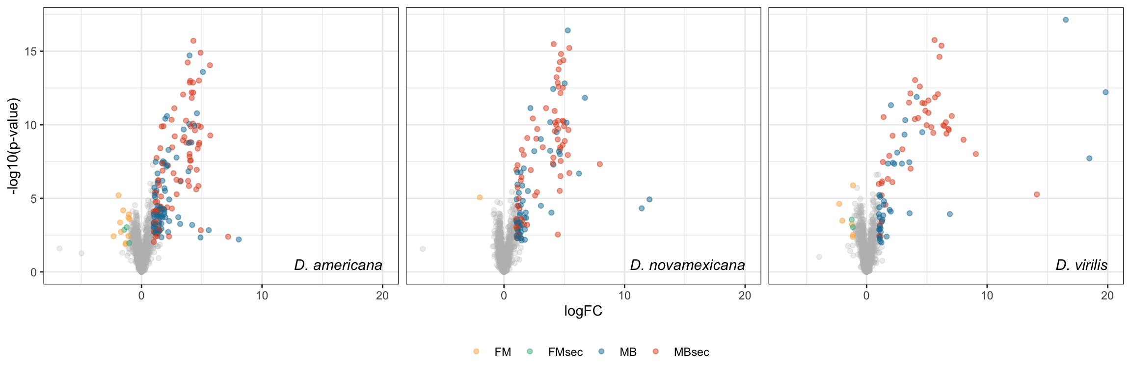
Overlap of ejaculate candidates between species
# #comb db
# upset(fromList(list(ame = comb_TABLES_nd$Orthogroup[comb_TABLES_nd$species == 'ame' & comb_TABLES_nd$logFC > 1 & comb_TABLES_nd$adj.P.Val < 0.05],
#                     nov = comb_TABLES_nd$Orthogroup[comb_TABLES_nd$species == 'nov' & comb_TABLES_nd$logFC > 1 & comb_TABLES_nd$adj.P.Val < 0.05],
#                     vir = comb_TABLES_nd$Orthogroup[comb_TABLES_nd$species == 'vir' & comb_TABLES_nd$logFC > 1 & comb_TABLES_nd$adj.P.Val < 0.05])))

#pdf('plots/TPP_results/TPP_sfp_overlap.pdf', height = 4, width = 4)
plot(venn(c('D. ame' = 46, "D. nov" = 18, "D. vir" = 13,
            'D. ame&D. nov' = 31, 'D. ame&D. vir' = 5, 'D. nov&D. vir' = 1,
            'D. ame&D. nov&D. vir' = 55)),
     quantities = TRUE,
     fills = list(fill = viridis::viridis(n = 3), alpha = .5))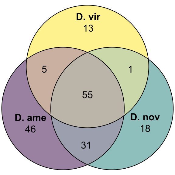
#dev.off()

# # percent overlap
# comb_TABLES_nd %>%
#   filter(logFC > 1, adj.P.Val < 0.05) %>%
#   group_by(species) %>%
#   count() %>%
#   mutate(p = 55/n * 100)

# proportion of ejaculate candidates with signal peptide
comb_TABLES_nd %>%
  filter(str_detect(DA, pattern = 'MB')) %>%
  distinct(genes, species, .keep_all = TRUE) %>%
  group_by(species, DA) %>% dplyr::count() %>%
  pivot_wider(id_cols = species, names_from = DA, values_from = n) %>%
  mutate(prop.sec = MBsec/(MBsec + MB)) %>%
  kable(digits = 3,
        caption = 'The number of proteins higher in abundance in mated comapred to virgin samples with or without a secretion signal for each species') %>%
kable_styling(full_width = FALSE)| species | MB | MBsec | prop.sec |
|---|---|---|---|
| ame | 77 | 84 | 0.522 |
| nov | 55 | 66 | 0.545 |
| vir | 38 | 46 | 0.548 |
Sfp overlap with previous studies
We compare the number of putative seminal fluid proteins identified in previous studies in the virilis group from Ahmed-Braimah et al. 2017 and Ahmed-Braimah et al. 2021.
overlap with Ahmed-Braimah et al. 2017
# upset(fromList(list(proteomic = ejac_cands_multiDB$FBgn,
#                     AG_biased = Dvir_SFPs$FBgn[Dvir_SFPs$bias == 'AG-biased'],
#                     EB_biased = Dvir_SFPs$FBgn[Dvir_SFPs$bias == 'EB-biased'],
#                     SFP       = Dvir_SFPs$FBgn[Dvir_SFPs$bias == 'SFP'])))

#pdf('plots/TPP_sfp_orth_overlap.pdf', height = 4, width = 4)
plot(euler(c('AG' = 107, "EB" = 85, "Prot" = 196, 'SFP' = 49,
             'SFP&Prot' = 22, 'AG&Prot' = 12, 'EB&Prot' = 7)),
     quantities = TRUE,
     fills = list(fill = c("turquoise", "orange", "red", 'purple'), alpha = .5))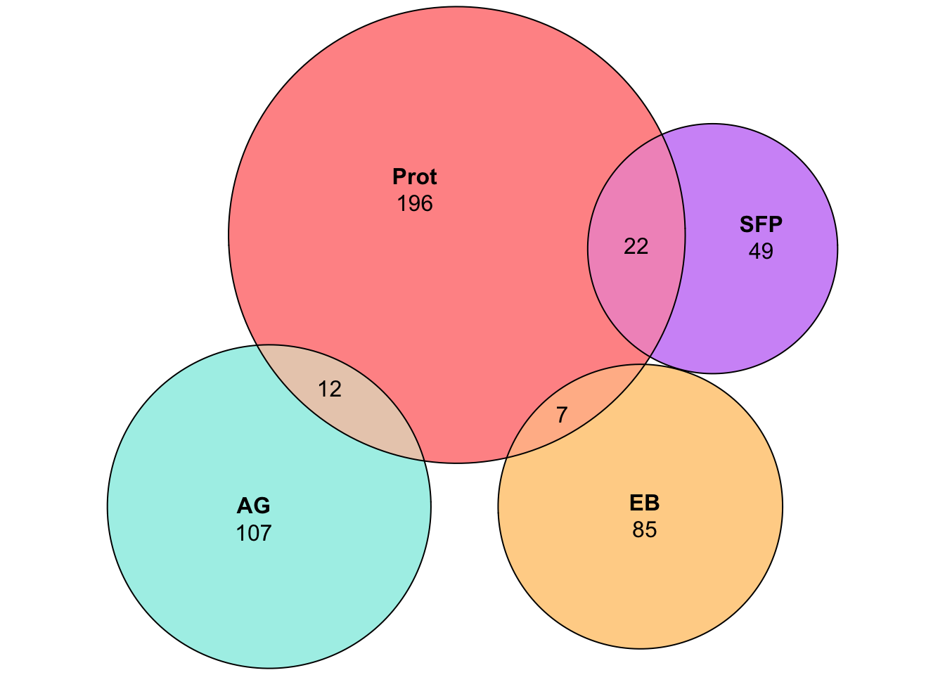
#dev.off()Overlap with female reproductive tract genes
# upset(fromList(list(proteomic = unique(comb_TABLES$FBgn),
#                     FRT_biased = FRTbiased$FBgn_ID,
#                     PMR_biased = virilisPMDE$FBgn_ID)))

plot(euler(c('FRT' = 84, "PMR" = 334, "PRO" = 2031,
             'FRT&PMR' = 14, 'FRT&PRO' = 48, 'PRO&PMR' = 93,
             'FRT&PMR&PRO' = 2)
              ),
     quantities = TRUE,
     fills = list(fill = c("orange", "red", 'purple'), alpha = .5))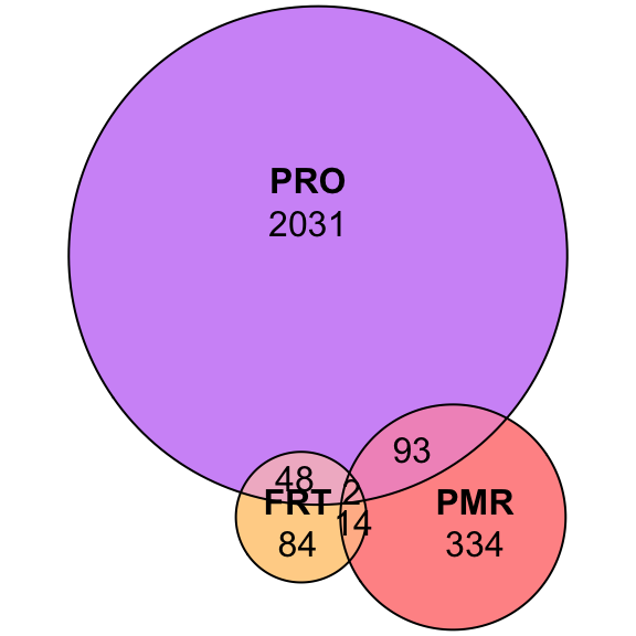
Detecting artifactual differences
We look at potential differences in abundance between groups of proteins which may indicate flaws in the experimental design. For instance, ejaculate proteins may be ‘swamped out’ by the more highly abundant/speciose female reproductive tract proteins. Furthermore, serine-type endopeptidases (STEP) are down-regulated after mating - a signature of the postmating female response. If our method is effective at capturing the female reproductive tract in a ‘virgin-like’ state, then we expect no difference in the abundance of STEPs between mated and virgin samples.
Abundance of ejaculate proteins compared to remaining FRT proteins
wilc_abund <- comb_TABLES_nd %>%
  mutate(up = if_else(adj.P.Val < 0.05 & logFC > 1, "ejac", 'frt')) %>%
  group_by(species) %>%
  do(fit = broom::tidy(wilcox.test(AveExpr ~ as.factor(up), data = .))) %>%
  unnest(fit) %>%
  mutate(up = NA,
         p.val = ifelse(p.value < 0.001, "p < 0.001", paste0('p = ', round(p.value, 3))))

comb_TABLES_nd %>%
  mutate(up = if_else(adj.P.Val < 0.05 & logFC > 1, "Ejaculate", 'FRT')) %>%
  ggplot(aes(x = up, y = AveExpr)) +
  geom_violin(aes(fill = up), alpha = .5) +
  geom_boxplot(aes(fill = up), width = .3, notch = TRUE) +
  geom_jitter(data = comb_TABLES_nd %>%
                mutate(up = if_else(adj.P.Val < 0.05 & logFC > 1, "Ejaculate", 'FRT')) %>%
                filter(up == 'Ejaculate'),
              colour = cbPalette[8], width = .3, alpha = .5) +
  # gghalves::geom_half_boxplot(aes(fill = up), outlier.shape = NA) +
  # gghalves::geom_half_point(aes(colour = up), alpha = .3) +
  scale_fill_manual(values = cbPalette[8:9]) +
  scale_colour_manual(values = cbPalette[8:9]) +
  facet_wrap(~species, nrow = 1, labeller = as_labeller(facet_names)) +
  labs(y = 'Average abundance') +
  theme_bw() +
  theme(legend.position = '',
        axis.title.x = element_blank(),
        strip.text = element_text(size = 15, face = "italic")) +
  geom_text(data = wilc_abund,
            aes(x = 1.5, y = 12,
                label = #paste0('Chi^2(1) = ', round(statistic, 2),
                        #       ', ',
                  p.val)) +
  # ggsignif::geom_signif(comparisons = list(c("ejac", "frt")),
  #                       map_signif_level = TRUE) +
  #ggsave('plots/TPP_results/TPP_ejac_vs_frt.pdf', height = 4, width = 12, dpi = 600, useDingbats = FALSE) +
  NULL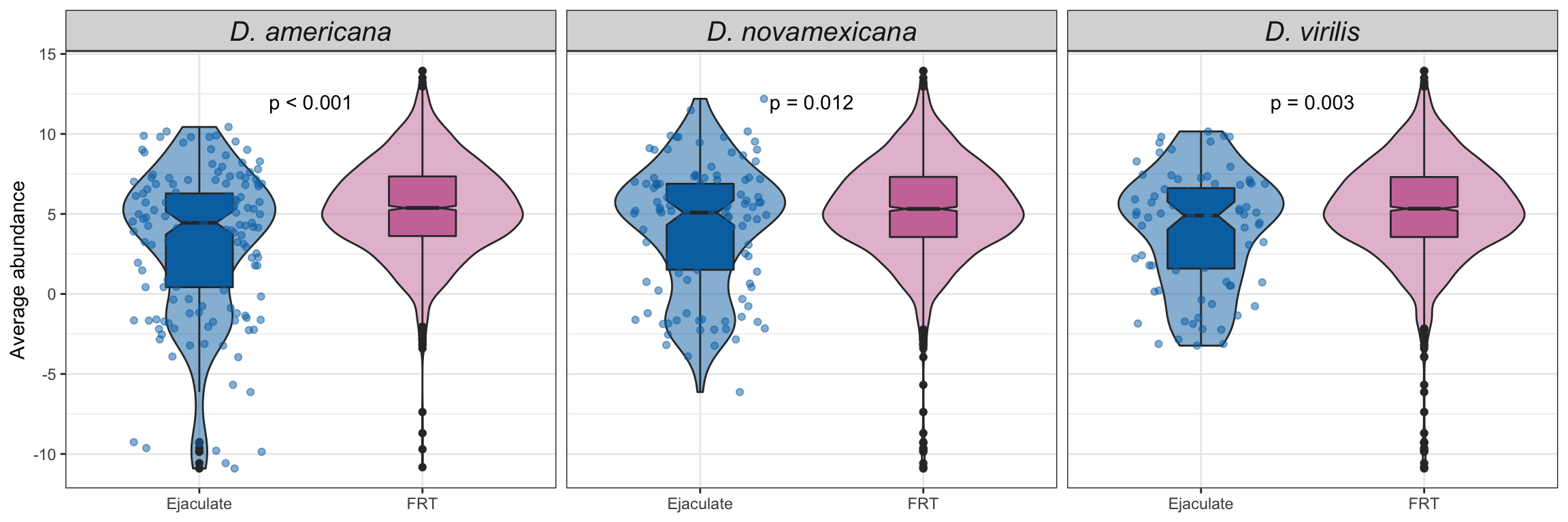
Abundance of serine-type endopeptidases
We downloaded gene ontology (GO) information for all D. virilis genes from FlyBase.org and identified all genes with serine-type endopeptidase (STEP) annotation. We tested whether these STEPs differed in abundance between samples using Kruskal-Wallis rank sum tests.
wilc_STEP <- comb_TABLES_nd %>%
  mutate(up = if_else(adj.P.Val < 0.05 & logFC > 1, "Ejaculate", 'FRT')) %>%
  filter(FBgn %in% STEP$FBgn) %>%
  group_by(species) %>%
  do(fit = broom::tidy(wilcox.test(AveExpr ~ as.factor(up), data = .))) %>%
  unnest(fit) %>%
  mutate(up = NA,
         p.val = ifelse(p.value < 0.001, "p < 0.001", paste0('p = ', round(p.value, 3))))

comb_TABLES_nd %>%
  mutate(up = if_else(adj.P.Val < 0.05 & logFC > 1, "Ejaculate", 'FRT')) %>%
  filter(FBgn %in% STEP$FBgn) %>%
  ggplot(aes(x = up, y = AveExpr, fill = up)) +
  gghalves::geom_half_boxplot(aes(fill = up), outlier.shape = NA) +
  gghalves::geom_half_point(aes(colour = up), alpha = .3) +
  scale_fill_manual(values = cbPalette[8:9]) +
  scale_colour_manual(values = cbPalette[8:9]) +
  labs(y = 'Average abundance') +
  facet_wrap(~species, nrow = 1, labeller = as_labeller(facet_names)) +
  theme_bw() +
  theme(legend.position = '',
        axis.title.x = element_blank(),
        strip.text = element_text(size = 15, face = "italic")) +
  geom_text(data = wilc_STEP,
            aes(x = 1.5, y = 11,
                label = p.val)) +
  # ggsignif::geom_signif(comparisons = list(c("Ejaculate", "FRT")),
  #                       map_signif_level = TRUE) +
  #ggsave('plots/TPP_results/TPP_STEP_abundance.pdf', height = 3, width = 9, dpi = 600, useDingbats = FALSE) +
  NULL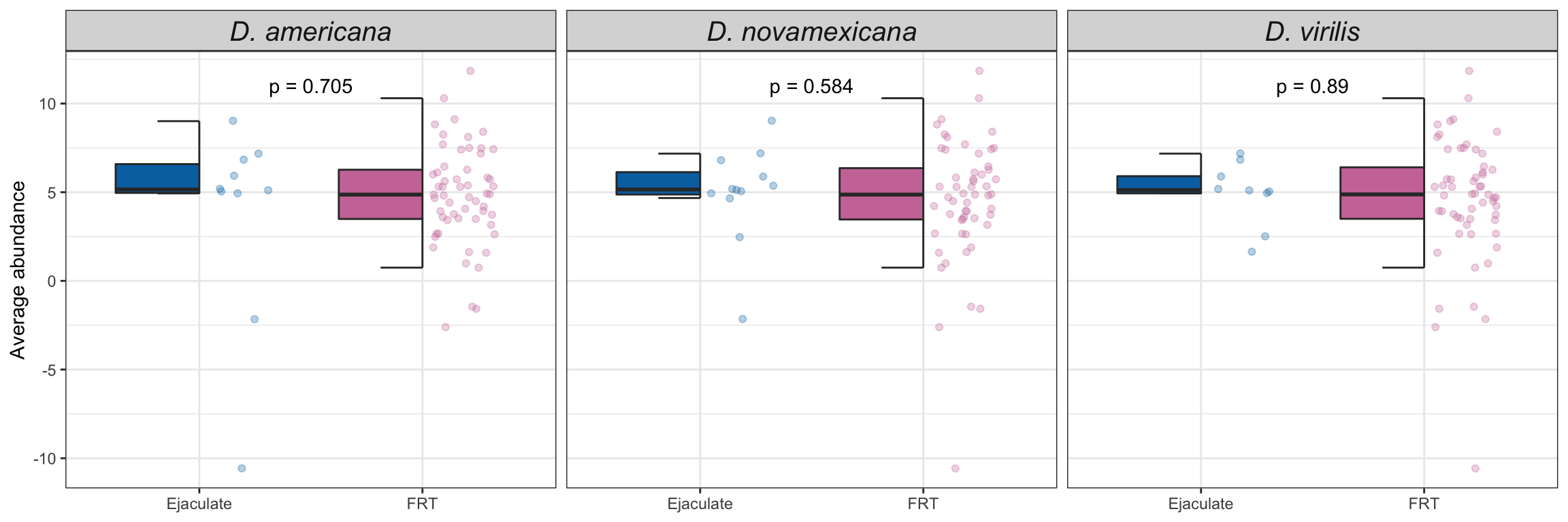
We replot the volcano plots to highlight serine-type endopeptidases, postmating female response genes and female reproductive tract genes perturbed after a heterospecific mating.
comb_TABLES %>%
  ggplot(aes(x = logFC, y = -log10(P.Value))) +
  geom_point(alpha = .1) +
  scale_colour_manual(values = c('red', 'hotpink', 'blue', 'purple', 'grey90')) +
  geom_point(data = comb_TABLES %>%
    filter(threshold == 'SD' & FBgn %in% STEP$FBgn), colour = 'yellow', alpha = .8, size = 3) +
  geom_point(data = comb_TABLES %>%
    filter(threshold == 'SD' & FBgn %in% FRTbiased$FBgn_ID), colour = 'blue', alpha = .8, size = 3) +
  geom_point(data = comb_TABLES %>%
    filter(threshold == 'SD' & FBgn %in% virilisPMDE$FBgn_ID), colour = 'green', alpha = .8, size = 3) +
  facet_wrap(~species) +
  theme_bw() +
  theme(strip.text = element_text(size = 15, face = "italic")) +
  NULL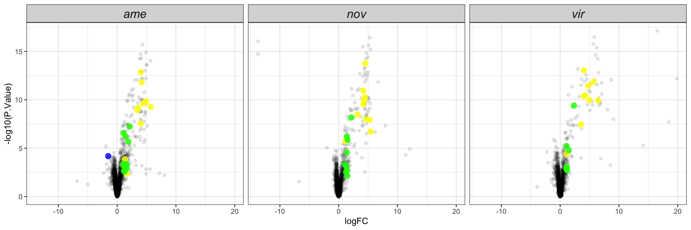
# #### Abundance of female reproductive tract biased genes and postmating female response genes
# upset(fromList(list(proteomic = comb_TABLES$FBgn,
#                     FRT_biased = FRTbiased$FBgn_ID,
#                     PMR_biased = virilisPMDE$FBgn_ID)))
#
# comb_TABLES %>% filter(FBgn %in% FRTbiased$FBgn_ID & threshold == 'SD')
# comb_TABLES %>% filter(FBgn %in% virilisPMDE$FBgn_ID & threshold == 'SD') %>% distinct(genes, .keep_all = TRUE)
#
# intersect(comb_TABLES_nd %>% filter(FBgn %in% FRTbiased$FBgn_ID & threshold == 'SD') %>% pull(genes),
#           comb_TABLES_nd %>% filter(FBgn %in% virilisPMDE$FBgn_ID & threshold == 'SD') %>% pull(genes))
#
# # STEP showing differences in abundance
# comb_TABLES %>%
#     filter(threshold == 'SD' & FBgn %in% STEP$FBgn) %>% distinct(genes, .keep_all = TRUE)
Divergence between ejaculate candidates
We tested for differential abundance of proteins found in mated samples between each species. We restrict the data to those proteins which showed differential abundance between mated and virgin samples (adjusted p-value < 0.05 and logFC > |1|) in any species, i.e. putative male derived/Sfps/sperm proteins.
sfp_dat <- multiDB %>%
  filter(protein_vir %in% unique(comb_TABLES %>% filter(adj.P.Val < 0.05  & logFC > 1) %>% pull(genes))) %>%
  select(Orthogroup, protein_vir, contains('M')) %>%
  mutate(across(3:11, ~replace_na(.x, 0)))

# make design matrix to test diffs between groups
matedSample <- sampInfo$condition[grep('M', x = sampInfo$condition)]
matedDesign <- model.matrix(~0 + matedSample)
colnames(matedDesign) <- unique(matedSample)
rownames(matedDesign) <- rep(1:3, 3)

# create DGElist and fit model
dgeSFP <- DGEList(counts = sfp_dat[, -c(1:2)], genes = sfp_dat$protein_vir, group = matedSample)
dgeSFP <- calcNormFactors(dgeSFP, method = 'TMM')
dgeSFP <- estimateCommonDisp(dgeSFP)
dgeSFP <- estimateTagwiseDisp(dgeSFP)
# voom normalisation
dgeSFPvoom <- voom(dgeSFP, matedDesign, plot = FALSE)
# fit linear model
lmSFP <- lmFit(dgeSFPvoom, design = matedDesign)

# make contrasts - higher values = higher in first alphabetically
cont.mated <- makeContrasts(ame.MTD.nov = AM - NM,
                            ame.MTD.vir = AM - VM,
                            nov.MTD.vir = NM - VM,
                            levels = matedDesign)

# perform lmFit tests
# ame vs. nov
lm_anM <- contrasts.fit(lmSFP, cont.mated[,"ame.MTD.nov"])
lm_anM <- eBayes(lm_anM)
lm_anM.tTags.table <- topTable(lm_anM, adjust.method = "BH", number = Inf) %>%
  mutate(comparison = "aMn",
         threshold = if_else(adj.P.Val < 0.05 & abs(logFC) > 1, "SD", "NS"))

# ame vs. vir
lm_avM <- contrasts.fit(lmSFP, cont.mated[,"ame.MTD.vir"])
lm_avM <- eBayes(lm_avM)
lm_avM.tTags.table <- topTable(lm_avM, adjust.method = "BH", number = Inf) %>%
  mutate(comparison = "aMv",
         threshold = if_else(adj.P.Val < 0.05 & abs(logFC) > 1, "SD", "NS"))

# nov vs. vir
lm_nvM <- contrasts.fit(lmSFP, cont.mated[,"nov.MTD.vir"])
lm_nvM <- eBayes(lm_nvM)
lm_nvM.tTags.table <- topTable(lm_nvM, adjust.method = "BH", number = Inf) %>%
  mutate(comparison = "nMv",
         threshold = if_else(adj.P.Val < 0.05 & abs(logFC) > 1, "SD", "NS"))

mated_TABLES <- rbind(lm_anM.tTags.table,
                      lm_avM.tTags.table,
                      lm_nvM.tTags.table) %>%
  left_join(vir_fbgn %>% select(-FBtr), by = c('genes' = 'gene_id')) %>%
  mutate(
    # add variable for signal peptides reaching significance threshold
    sigP = if_else(genes %in% vir_sig$protein, 'sigP', 'not'),
    # add variable splitting by bias to virgin vs. mated and signal peptide
    sperm = if_else(FBgn %in% sperm_mel$FBgn_v, 'Sperm', 'not'),
    Sfp = if_else(FBgn %in% wigbySFP$FBgn, 'Sfp', 'not'),
    DA = case_when(is.na(genes) == TRUE & threshold == 'SD' ~ "uni",
                   sigP == 'sigP' & threshold == 'SD' ~ "sigP",
                   threshold == 'SD' ~ "DA",
                   TRUE ~ 'NS')) %>%
  distinct(genes, comparison, .keep_all = TRUE)

# remove duplicated genes
mated_TABLES_nd <- mated_TABLES %>% filter(!Orthogroup %in% ortho_dups$Orthogroup)

# #save differentially abundant proteins to table for ClueGO
# mated_TABLES %>% filter(threshold == 'SD') %>%
#   distinct(FBgn, .keep_all = TRUE) %>% write_csv('output/ClueGOlists/TPP_Sfp_DA_multiDB.csv')
MA plots
mated_TABLES_nd %>% filter(DA != 'NS') %>%
  ggplot(aes(x = AveExpr, y = logFC, colour = DA)) +
  geom_point(data = mated_TABLES_nd %>% filter(DA == 'NS'), colour = 'grey') +
  geom_point(alpha = .6) +
  geom_point(data = mated_TABLES %>%
               filter(Orthogroup %in% ortho_dups$Orthogroup, threshold == "SD"),
             colour = "red") +
  scale_colour_manual(values = egypt.pal) +
  labs(y = '-log10(p-value)') +
  facet_wrap(~comparison, nrow = 1,
             labeller = as_labeller(c(aMn = "D. americana vs. D. novamexicana",
                                      aMv = 'D. americana vs. D. virilis',
                                      nMv = "D. novamexicana vs. D. virilis"))) +
  theme_bw() +
  theme(legend.position = c(0.04, 0.2),
        legend.background = element_rect(fill = NA),
        legend.title = element_blank(),
        strip.text = element_text(size = 15, face = "italic")) +
  # geom_label_repel(
  #   data = mated_TABLES_nd %>% filter(DA != 'NS') %>% left_join(wigbySFP, by = 'FBgn'),
  #   aes(label = Symbol),
  #   size = 4,
  #   colour = 'black',
  #   box.padding = unit(0.35, "lines"),
  #   point.padding = unit(0.3, "lines")
  # ) +
  #ggsave('plots/TPP_results/MA_sfp.pdf', height = 4, width = 12, dpi = 600, useDingbats = FALSE) +
  NULL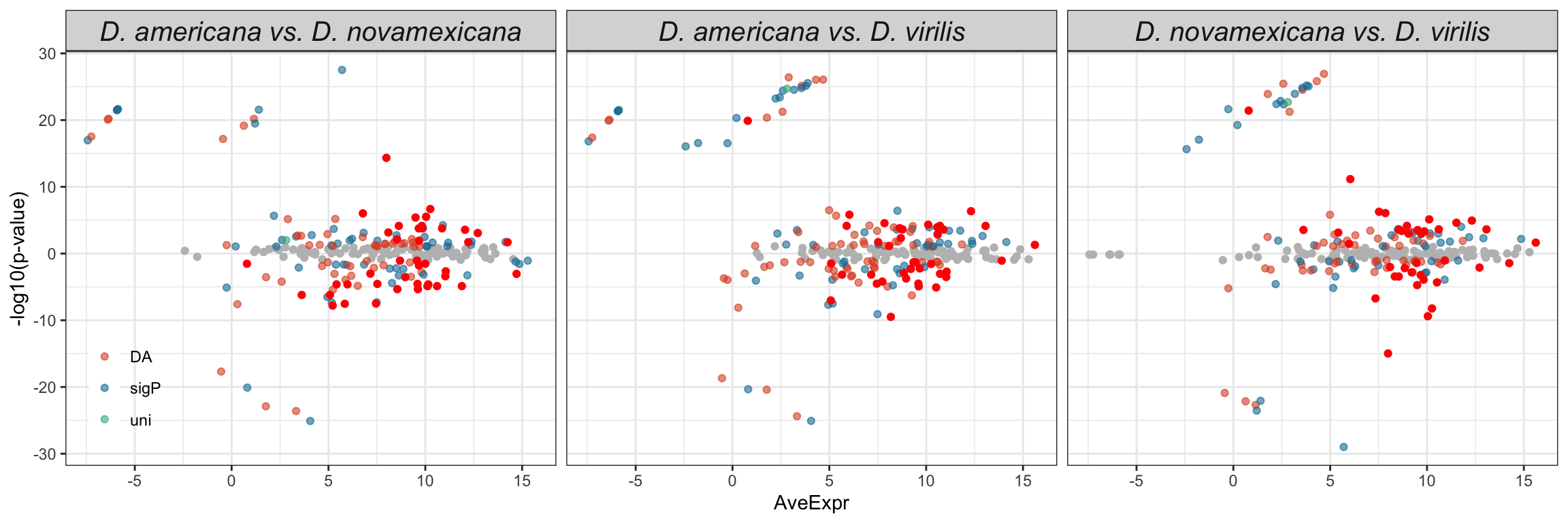
# total number of SFPs differentially abundant
mated_TABLES %>% filter(threshold == "SD") %>%
  left_join(wigbySFP, by = 'FBgn') %>% drop_na(Symbol) %>% pull(Symbol) %>% unique()
[1] "Est-6" "CG15117" "NT5E-2" "CG2852" "scpr-A" "CG40160" "CG11977"
[8] "aqrs" "CG34002" "CG17574" "Hexo2" "CG34129" "CG42564" "Npc2b"
[15] "CG14034" "CG4815" # number of copies differentially abundant in each comparison
mated_TABLES %>% filter(threshold == "SD") %>%
left_join(wigbySFP, by = 'FBgn') %>% drop_na(Symbol) %>%
group_by(comparison, Symbol) %>%
count() %>% pivot_wider(names_from = comparison, values_from = n)# A tibble: 16 × 4
# Groups: Symbol [16]
Symbol aMn aMv nMv
<chr> <int> <int> <int>
1 aqrs 1 1 NA
2 CG11977 1 1 NA
3 CG15117 1 1 1
4 CG17574 1 1 1
5 CG2852 1 NA 1
6 CG34002 1 1 1
7 CG34129 1 NA 1
8 CG40160 1 1 NA
9 CG42564 1 1 1
10 Est-6 1 1 NA
11 Hexo2 1 1 NA
12 NT5E-2 1 1 1
13 scpr-A 3 3 3
14 CG14034 NA 1 1
15 CG4815 NA 1 1
16 Npc2b NA 1 1# table of all differentially abundant SFPs or sperm proteins
bind_rows(mated_TABLES %>% filter(threshold == "SD") %>%
left_join(wigbySFP, by = 'FBgn') %>%
distinct(FBgn_mel, .keep_all = TRUE) %>% drop_na(Symbol) %>%
select(FBgn, FBgn_mel, Symbol),
mated_TABLES %>% filter(threshold == "SD") %>%
left_join(sperm_mel, by = c("FBgn" = "FBgn_v")) %>%
distinct(mel_FBgn_ID, .keep_all = TRUE) %>% drop_na(mel_FBgn_ID) %>%
select(FBgn, FBgn_mel = mel_FBgn_ID, Symbol = Gene.Symbol)) %>%
#write_csv()
kable(caption = 'D. melanogaster SFPs and sperm protein orthologs showing differential abundannce between ejaculate candidates') %>%
kable_styling(full_width = FALSE) %>%
group_rows("SFPs", 1, 13) %>%
group_rows("Sperm proteins", 14, 26)| FBgn | FBgn_mel | Symbol |
|---|---|---|
| SFPs | ||
| FBgn0197362 | FBgn0000592 | Est-6 |
| FBgn0206811 | FBgn0034417 | CG15117 |
| FBgn0207519 | FBgn0050104 | NT5E-2 |
| FBgn0208385 | FBgn0034753 | CG2852 |
| FBgn0211755 | FBgn0037889 | scpr-A |
| FBgn0211457 | FBgn0058160 | CG40160 |
| FBgn0204606 | FBgn0037650 | CG11977 |
| FBgn0211264 | FBgn0039598 | aqrs |
| FBgn0208251 | FBgn0054002 | CG34002 |
| FBgn0207308 | FBgn0033777 | CG17574 |
| FBgn0206035 | FBgn0041629 | Hexo2 |
| FBgn0210455 | FBgn0083965 | CG34129 |
| FBgn0211681 | FBgn0260766 | CG42564 |
| Sperm proteins | ||
| FBgn0211705 | FBgn0038198 | Npc2b |
| FBgn0204528 | FBgn0250847 | CG14034 |
| FBgn0211573 | FBgn0039568 | CG4815 |
| FBgn0202308 | FBgn0001187 | Hex-C |
| FBgn0210522 | FBgn0037891 | CG5214 |
| FBgn0204802 | FBgn0069354 | Porin2 |
| FBgn0016474 | FBgn0004045 | Yp1 |
| FBgn0199705 | FBgn0046704 | Liprin-alpha |
| FBgn0197452 | FBgn0013812 | Dhc93AB |
| FBgn0204735 | FBgn0031869 | CG18304 |
| FBgn0198514 | FBgn0015278 | Pi3K68D |
| FBgn0203892 | FBgn0086907 | Cyt-c-d |
| FBgn0202027 | FBgn0030482 | CG1673 |
| FBgn0205934 | FBgn0031171 | CG1801 |
| FBgn0199271 | FBgn0051644 | CG31644 |
| FBgn0201010 | FBgn0266136 | Gyc76C |
| FBgn0210936 | FBgn0038395 | CG10407 |
| FBgn0204803 | FBgn0260453 | CG17140 |
| FBgn0211422 | FBgn0039257 | tnc |
Overlap between differentially abundant proteins
# upset(fromList(list(
#   a.vs.n = lm_anM.tTags.table$genes[lm_anM.tTags.table$threshold == 'SD'],
#   a.vs.v = lm_avM.tTags.table$genes[lm_avM.tTags.table$threshold == 'SD'],
#   n.vs.v = lm_nvM.tTags.table$genes[lm_nvM.tTags.table$threshold == 'SD'])))

#pdf('plots/TPP_results/TPP_divergence_overlap_comb.pdf', height = 4, width = 4)
plot(venn(c('a.vs.n' = 6, 'a.vs.v' = 8, 'n.vs.v' = 6,
             'a.vs.n&a.vs.v' = 46, 'a.vs.n&n.vs.v' = 39, 'a.vs.v&n.vs.v' = 29,
             'a.vs.n&a.vs.v&n.vs.v' = 64)),
     quantities = TRUE,
     fills = list(fill = cbPalette[2:4], alpha = .5))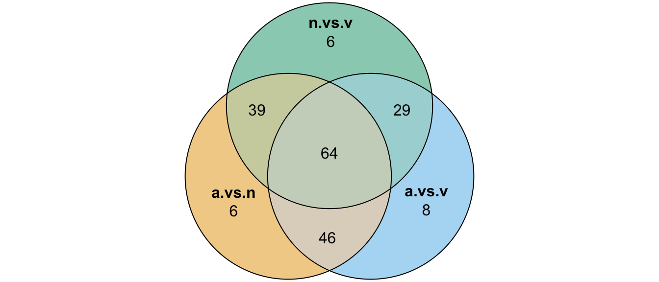
#dev.off()Are signal peps more likely to be differentially abundant?
mated_TABLES %>%
  group_by(comparison, threshold, sigP) %>% dplyr::count() %>%
  ggplot(aes(x = threshold, y = n, fill = sigP)) +
  geom_col(position = 'fill') +
  facet_wrap(~comparison, nrow = 1,
             labeller = as_labeller(c(aMn = "D. americana vs. D. novamexicana",
                                      aMv = 'D. americana vs. D. virilis',
                                      nMv = "D. novamexicana vs. D. virilis"))) +
  theme_bw() +
  NULL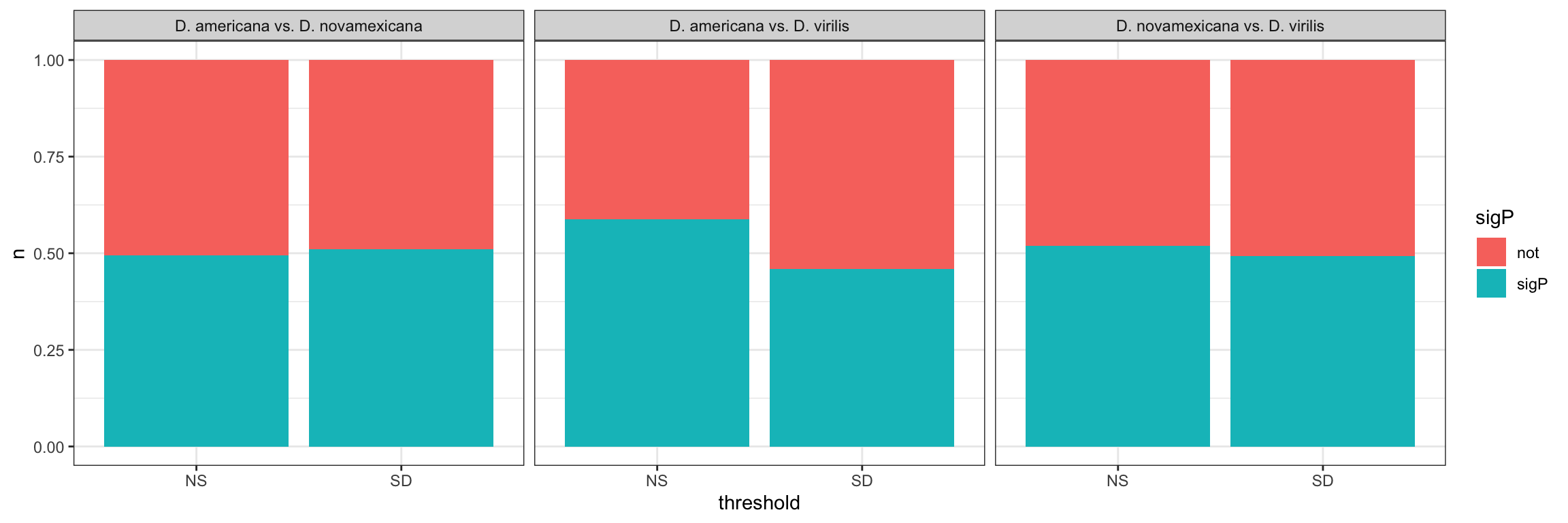
# Fisher's exact tests
mated_TABLES %>%
  group_by(comparison) %>%
  do(fit = broom::tidy(fisher.test(as.matrix(xtabs(~ threshold + sigP, ., sparse = TRUE))))) %>%
  unnest(fit) %>%
  mutate(comparison = recode(comparison,
                             aMn = "D. ame vs. D. nov",
                             aMv = "D. ame vs. D. vir",
                             nMv = 'D. nov vs. D. vir'),
         across(2:5, ~ round(.x, 2)),
         p.value = ifelse(p.value < 0.001, "< 0.001", p.value),
         Estimate = paste0(estimate, ' (', conf.low, '-', conf.high, ')')) %>%
  dplyr::select(Comparison = comparison, Estimate, p.value) %>%
  kable(caption = 'Fisher\'s exact tests for signal peptides that are differentially abundant or not') %>%
kable_styling(full_width = FALSE)| Comparison | Estimate | p.value |
|---|---|---|
| D. ame vs. D. nov | 1.06 (0.62-1.84) | 0.90 |
| D. ame vs. D. vir | 0.59 (0.34-1.05) | 0.06 |
| D. nov vs. D. vir | 0.9 (0.52-1.54) | 0.70 |
# are sperm genes more likely to be differentially abundant?
mated_TABLES %>%
  #filter(sperm == 'Sperm') %>%
  group_by(comparison, threshold, sperm) %>% dplyr::count() %>%
  ggplot(aes(x = sperm, y = n, fill = threshold)) +
  geom_col(position = 'fill') +
  facet_wrap(~comparison, nrow = 1,
             labeller = as_labeller(c(aMn = "D. americana vs. D. novamexicana",
                                      aMv = 'D. americana vs. D. virilis',
                                      nMv = "D. novamexicana vs. D. virilis"))) +
  theme_bw() +
  theme(strip.text = element_text(size = 15, face = "italic")) +
  NULL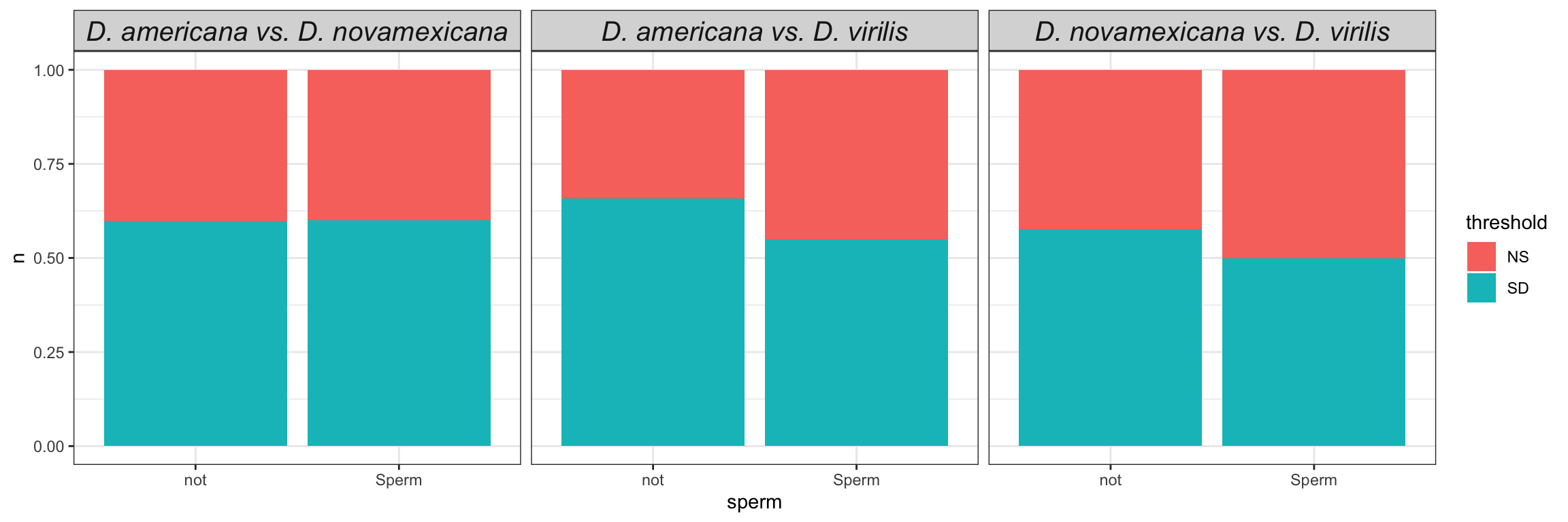
# Fisher's exact tests
mated_TABLES %>%
  group_by(comparison) %>%
  do(fit = broom::tidy(fisher.test(as.matrix(xtabs(~ threshold + sperm, ., sparse = TRUE))))) %>%
  unnest(fit) %>%
  mutate(across(2:5, ~ round(.x, 2)),
         p.value = ifelse(p.value < 0.001, '< 0.001', round(p.value, 3)),
         Estimate = paste0(estimate, ' (', conf.low, '-', conf.high, ')')) %>%
  dplyr::select(comparison, Estimate, p.value) %>%
  kable(digits = 3,
        caption = 'Fisher\'s exact tests for sperm proteins that are differentially abundant or not') %>%
kable_styling(full_width = FALSE)| comparison | Estimate | p.value |
|---|---|---|
| aMn | 1 (0.36-2.95) | 1.00 |
| aMv | 0.64 (0.23-1.82) | 0.34 |
| nMv | 0.74 (0.26-2.06) | 0.64 |
Heatmap
# make DF
sfp_md <- data.frame(dgeSFPvoom$genes,
                     dgeSFPvoom$E) %>%
  rowwise() %>%
  mutate(`D. ame` = median(c(!!! rlang::syms(grep('AM', names(.), value = TRUE)))),
         `D. nov` = median(c(!!! rlang::syms(grep('NM', names(.), value = TRUE)))),
         `D. vir` = median(c(!!! rlang::syms(grep('VM', names(.), value = TRUE))))) %>%
  #dplyr::select(genes, `D. ame`, `D. nov`, `D. vir`) %>%
  left_join(vir_fbgn %>% select(-FBtr), by = c('genes' = 'gene_id')) %>%
  # add mel Sfp ortholog
  left_join(wigbySFP %>% dplyr::select(FBgn, mel_Sfp = Symbol)) %>%
  mutate(Sfp = if_else(FBgn %in% wigbySFP$FBgn, 'Sfp', 'other'),
         category = case_when(FBgn %in% sperm_mel$FBgn_v ~ 'sperm',
                              FBgn %in% wigbySFP$FBgn ~ 'Sfp',
                              genes %in% vir_sig$protein ~ 'sigP',
                              TRUE ~ as.character(NA)),
         dupl = ifelse(Orthogroup %in% ortho_dups$Orthogroup, "Dupl", NA),
         orthdup = ifelse(dupl == "Dupl", Orthogroup, NA)) %>%
  distinct(genes, .keep_all = TRUE) #%>%
  # remove duplicated genes
  #filter(!Orthogroup %in% ortho_dups$Orthogroup)

sfp_hm <- sfp_md %>% select(`D. ame`, `D. nov`, `D. vir`,
                            FBgn, mel_Sfp, category)

#row.names(sfp_hm) <- sfp_md$genes

mat_scaled <- as.matrix(pheatmap:::scale_rows(sfp_hm[, 1:3]))

# # Dissimilarity matrix
# d <- dist(mat_scaled, method = "euclidean")
# # # Hierarchical clustering using Complete Linkage
# hc1 <- hclust(d, method = "complete" )
# # Plot the obtained dendrogram
# #plot(hc1, cex = 0.6, hang = -1)

fviz_nbclust(mat_scaled, FUN = hcut, method = "silhouette")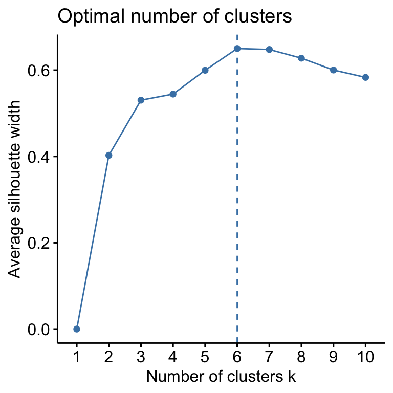
sub_grp <- kmeans(mat_scaled, centers = 6)$cluster

# # Cut tree into groups
# sub_grp <- cutree(hc1, k = 6)

# heatmap annotations
cat_lab <- rowAnnotation(Cluster = sub_grp,
                         col = list(Cluster = setNames(cbPalette[2:(max(sub_grp) + 1)], unique(sub_grp))),
                         title = NULL,
                         show_annotation_name = FALSE)

Sfp_labs <- rowAnnotation(#Dup_labs = sfp_md$orthdup,
                          Category = sfp_md$category,
                          col = list(Category = c(sperm = "blue",
                                                  Sfp = "purple",
                                                  sigP = "yellow"),
                                     Dup_labs = setNames(rep(viridis::turbo(
                                       n_distinct(sfp_md$orthdup[is.na(sfp_md$dupl) == FALSE])),
                                       rle(sfp_md$Orthogroup[is.na(sfp_md$dupl) == FALSE])$lengths),
                                       sfp_md$Orthogroup[is.na(sfp_md$dupl) == FALSE])),
                          na_col = NA,
                          Sfp_labs = anno_mark(at = c(grep('Sfp', x = sfp_md$Sfp)),
                                               labels = sfp_md$mel_Sfp[sfp_md$Sfp == 'Sfp'],
                                               labels_gp = gpar(fontsize = 8)),
                          title = NULL,
                          #show_legend = c("Dup_labs" = FALSE),
                          show_annotation_name = FALSE)

sfpha <- HeatmapAnnotation(species = anno_block(gp = gpar(fill = c(v.pal[c(3, 2, 1)])),
                                                labels = c(expression(italic('D. ame')),
                                                           expression(italic('D. nov')),
                                                           expression(italic('D. vir'))),
                                                labels_gp = gpar(col = c('white', 'white', 'black'),
                                                                 fontsize = 10)))

sfp_chm <- Heatmap(mat_scaled,
                   col = viridis::inferno(50),
                   heatmap_legend_param = list(title = "log2(intensities)",
                                               #title_position = "leftcenter-rot",
                                               direction = "horizontal",
                                               at = c(-1.5, 0, 1.5)),
                   right_annotation = Sfp_labs,
                   left_annotation = cat_lab,
                   top_annotation = sfpha,
                   show_row_names = FALSE,
                   show_column_names = FALSE,
                   row_split = max(sub_grp),
                   #row_km = max(sub_grp),
                   cluster_rows = cluster_within_group(t(mat_scaled), sub_grp),
                   column_split = 3,
                   column_gap = unit(0, "mm"),
                   row_title = NULL,
                   column_title = NULL)
#pdf('plots/TPP_results/TPP_sfp_heatmap.pdf', height = 8, width = 5)
sfp_chm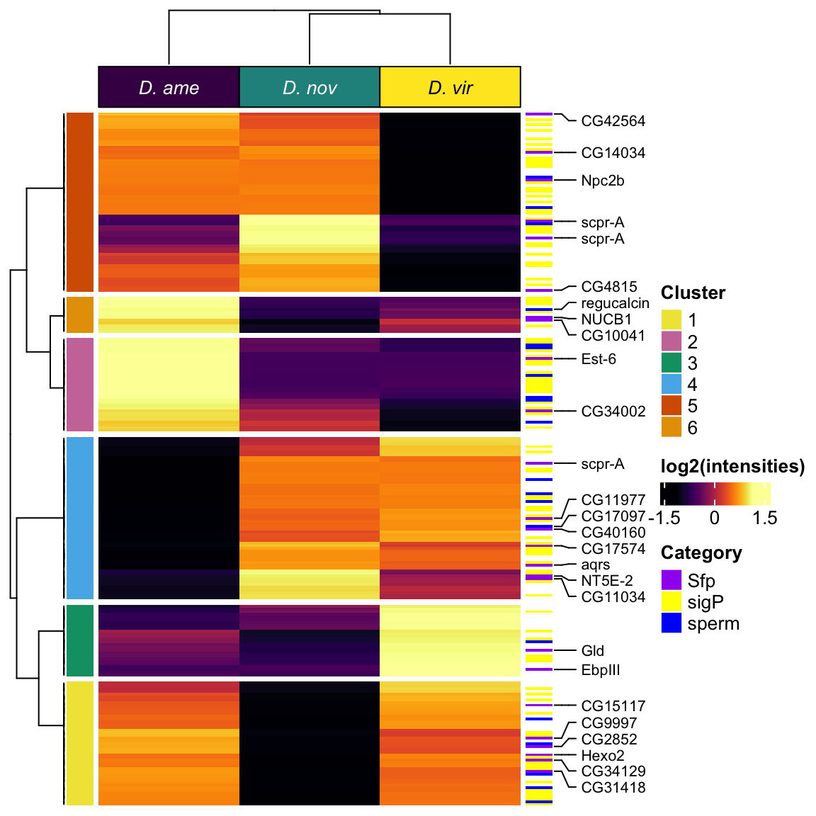
#dev.off()We tested how protein abundance differed between species based on k-means cluster
sfp_cluster <- data.frame(genes = sfp_md$genes, sfp_hm[, 1:3], cluster = sub_grp) %>%
  pivot_longer(cols = 2:4) %>%
  # #exclude proteins absent from each species (edgeR gives v. low estimate of abundance)
  #filter(value > -10) %>%
  mutate(species = str_sub(name, 4, 4))

sfp_cluster %>%
  mutate(cluster = paste('Cluster', cluster, sep = ' ')) %>%
  #ggplot(aes(x = factor(name, levels = c('D..vir', 'D..ame', 'D..nov')), y = value, fill = name)) +
  ggplot(aes(x = name, y = value, fill = name)) +
  gghalves::geom_half_point(aes(colour = name)) +
  gghalves::geom_half_violin(aes(fill = name)) +
  stat_pointinterval(pch = 21, fill = 'white') +
  labs(x = 'Species', y = 'normalised abundance') +
  scale_fill_viridis_d() +
  scale_colour_viridis_d() +
  facet_wrap(~cluster, scales = 'free_y') +
  theme_bw() +
  theme(legend.position = '',
        axis.text.x = element_text(face = 'italic')) +
  ggpubr::stat_compare_means(aes(label = ..p.signif..),
                             comparisons = list(c('D..ame', 'D..nov'),
                                                c('D..ame', 'D..vir'),
                                                c('D..nov', 'D..vir')),
                             method = 't.test') +
  #ggsave('plots/TPP_results/sfp_pointinterval.pdf', height = 6, width = 6, dpi = 600, useDingbats = FALSE) +
  NULL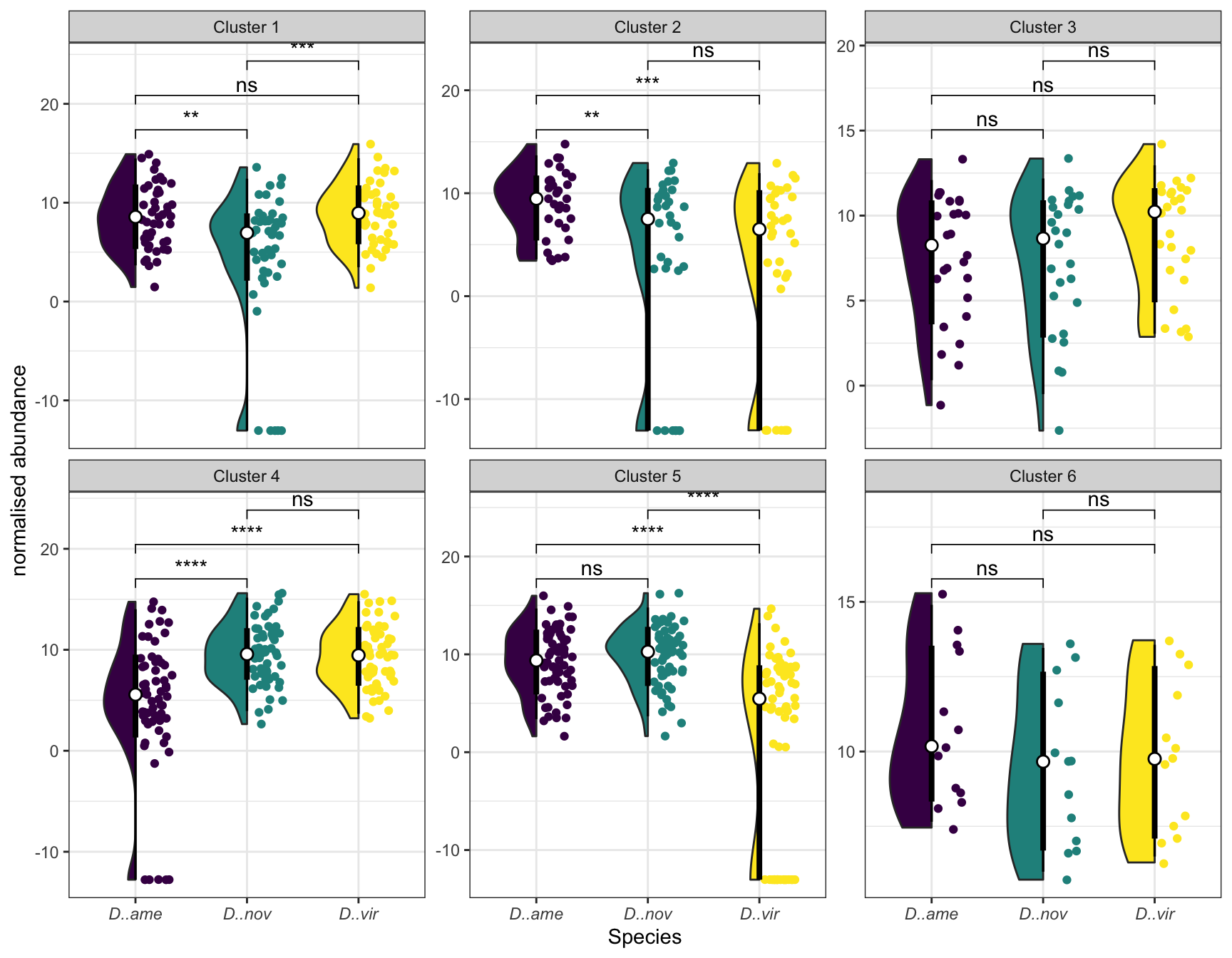
Model fits
sfp_cluster %>% group_by(cluster) %>%
  do(fit = broom::glance(lm(value ~ name, data = .))) %>%
  unnest(fit) %>%
  mutate(p.value = ifelse(p.value < 0.001, '< 0.001', round(p.value, 3))) %>%
  dplyr::select(-adj.r.squared, -sigma, -c(df:nobs)) %>%
  kable(digits = 3,
        caption = 'Model fits') %>%
kable_styling(full_width = FALSE)| cluster | r.squared | statistic | p.value |
|---|---|---|---|
| 1 | 0.140 | 10.724 | < 0.001 |
| 2 | 0.112 | 6.249 | 0.003 |
| 3 | 0.035 | 1.356 | 0.264 |
| 4 | 0.196 | 21.195 | < 0.001 |
| 5 | 0.293 | 39.701 | < 0.001 |
| 6 | 0.045 | 0.851 | 0.436 |
sfp_cluster %>% group_by(cluster) %>%
  do(fit = broom::tidy(lm(value ~ name, data = .))) %>%
  unnest(fit) %>%
  mutate(p.value = ifelse(p.value < 0.001, '< 0.001', round(p.value, 3)),
         sigLabel = case_when(p.value < 0.001 ~ "***",
                              p.value < 0.01 ~ "**",
                              p.value < 0.05 ~ "*",
                              TRUE ~ '')) %>%
  kable(digits = 3,
        caption = 'Model estimates') %>%
kable_styling(full_width = FALSE)| cluster | term | estimate | std.error | statistic | p.value | sigLabel |
|---|---|---|---|---|---|---|
| 1 | (Intercept) | 8.526 | 0.719 | 11.861 | < 0.001 | *** |
| 1 | nameD..nov | -3.915 | 1.017 | -3.852 | < 0.001 | *** |
| 1 | nameD..vir | 0.306 | 1.017 | 0.301 | 0.764 | |
| 2 | (Intercept) | 9.052 | 1.300 | 6.962 | < 0.001 | *** |
| 2 | nameD..nov | -5.341 | 1.839 | -2.904 | 0.005 | ** |
| 2 | nameD..vir | -5.881 | 1.839 | -3.198 | 0.002 | ** |
| 3 | (Intercept) | 7.540 | 0.729 | 10.335 | < 0.001 | *** |
| 3 | nameD..nov | -0.214 | 1.032 | -0.207 | 0.836 | |
| 3 | nameD..vir | 1.353 | 1.032 | 1.311 | 0.194 | |
| 4 | (Intercept) | 4.747 | 0.586 | 8.103 | < 0.001 | *** |
| 4 | nameD..nov | 4.751 | 0.829 | 5.734 | < 0.001 | *** |
| 4 | nameD..vir | 4.589 | 0.829 | 5.538 | < 0.001 | *** |
| 5 | (Intercept) | 9.321 | 0.761 | 12.249 | < 0.001 | *** |
| 5 | nameD..nov | 0.578 | 1.076 | 0.537 | 0.592 | |
| 5 | nameD..vir | -8.001 | 1.076 | -7.434 | < 0.001 | *** |
| 6 | (Intercept) | 10.730 | 0.722 | 14.861 | < 0.001 | *** |
| 6 | nameD..nov | -1.289 | 1.021 | -1.262 | 0.215 | |
| 6 | nameD..vir | -0.936 | 1.021 | -0.917 | 0.365 |
sfp_cluster %>% group_by(cluster) %>%
  do(fit = broom::tidy(TukeyHSD(aov(value ~ name, data = .)))) %>%
  unnest(fit) %>%
  mutate(contrast = recode(contrast,
                      `D. nov-D. ame` = "D. ame vs. D. nov",
                      `D. vir-D. ame` = "D. ame vs. D. vir",
                      `D. vir-D. nov` = 'D. nov vs. D. vir'),
         p.value = ifelse(adj.p.value < 0.001, '< 0.001', round(adj.p.value, 3)),
         across(4:8, ~ round(.x, 2)),
         Estimate = paste0(estimate, ' (', conf.low, '-', conf.high, ')'),
         sigLabel = case_when(p.value < 0.001 ~ "***",
                              p.value < 0.01 ~ "**",
                              p.value < 0.05 ~ "*",
                              TRUE ~ '')) %>%
  dplyr::select(-term, -null.value, -c(estimate:adj.p.value)) %>%
  kable(digits = 3,
        caption = 'Post hoc contrasts') %>%
kable_styling(full_width = FALSE)| cluster | contrast | p.value | Estimate | sigLabel |
|---|---|---|---|---|
| 1 | D..nov-D..ame | < 0.001 | -3.92 (-6.33–1.51) | *** |
| 1 | D..vir-D..ame | 0.951 | 0.31 (-2.1-2.72) | |
| 1 | D..vir-D..nov | < 0.001 | 4.22 (1.81-6.63) | *** |
| 2 | D..nov-D..ame | 0.013 | -5.34 (-9.72–0.97) |
|
| 2 | D..vir-D..ame | 0.005 | -5.88 (-10.26–1.5) | ** |
| 2 | D..vir-D..nov | 0.954 | -0.54 (-4.92-3.84) | |
| 3 | D..nov-D..ame | 0.977 | -0.21 (-2.68-2.25) | |
| 3 | D..vir-D..ame | 0.393 | 1.35 (-1.11-3.82) | |
| 3 | D..vir-D..nov | 0.288 | 1.57 (-0.9-4.03) | |
| 4 | D..nov-D..ame | < 0.001 | 4.75 (2.79-6.71) | *** |
| 4 | D..vir-D..ame | < 0.001 | 4.59 (2.63-6.55) | *** |
| 4 | D..vir-D..nov | 0.979 | -0.16 (-2.12-1.8) | |
| 5 | D..nov-D..ame | 0.853 | 0.58 (-1.96-3.12) | |
| 5 | D..vir-D..ame | < 0.001 | -8 (-10.54–5.46) | *** |
| 5 | D..vir-D..nov | < 0.001 | -8.58 (-11.12–6.04) | *** |
| 6 | D..nov-D..ame | 0.425 | -1.29 (-3.78-1.21) | |
| 6 | D..vir-D..ame | 0.633 | -0.94 (-3.43-1.56) | |
| 6 | D..vir-D..nov | 0.936 | 0.35 (-2.14-2.85) |
Divergence between (virgin) reproductive tracts
fem_dat <- multiDB %>%
  filter(!protein_vir %in% c(comb_TABLES %>% filter(adj.P.Val < 0.05  & logFC > 1) %>% pull(genes))) %>%
  #filter(!Orthogroup %in% c(ame_cands$Orthogroup, nov_cands$Orthogroup, vir_cands$Orthogroup)) %>%
  dplyr::select(-contains('M')) %>%
  mutate(across(3:9, ~replace_na(.x, 0)))

# # most identified sperm proteins remain in virgin samples after excluding DA proteins between mated/viring samples
# fem_dat %>%
#   left_join(vir_fbgn, by = c("protein_vir" = "gene_id", "Orthogroup")) %>%
#   distinct(protein_vir, .keep_all = TRUE) %>%
#   filter(FBgn %in% sperm_mel$FBgn_v)
#
# multiDB %>%
#   left_join(vir_fbgn, by = c("protein_vir" = "gene_id", "Orthogroup")) %>%
#   distinct(protein_vir, .keep_all = TRUE) %>%
#   filter(FBgn %in% sperm_mel$FBgn_v)

# # number of FRT proteins with...
# fem_dat %>% map_dbl(n_distinct)
# fem_dat %>% distinct(protein_vir) %>% filter(protein_vir %in% vir_sig$protein) %>% dim()

# make design matrix to test diffs between groups
femSample <- sampInfo$condition[grep('V$', x = sampInfo$condition)]
femdesign <- model.matrix(~0 + femSample)
colnames(femdesign) <- unique(femSample)
rownames(femdesign) <- c(rep(1:2, 2), 1:3)

# create DGElist and fit model
dgeFEM <- DGEList(counts = fem_dat[, -c(1:2)], genes = fem_dat$protein_vir, group = femSample)
dgeFEM <- calcNormFactors(dgeFEM, method = 'TMM')
dgeFEM <- estimateCommonDisp(dgeFEM)
dgeFEM <- estimateTagwiseDisp(dgeFEM)
# voom normalisation
dgeFEMvoom <- voom(dgeFEM, femdesign, plot = FALSE)
# fit linear model
lmFEM <- lmFit(dgeFEMvoom, design = femdesign)

# make contrasts - higher values = higher in first alphabetically
cont.fem <- makeContrasts(ame.FEM.nov = AV - NV,
                          ame.FEM.vir = AV - VV,
                          nov.FEM.vir = NV - VV,
                          levels = femdesign)

# perform lmFit tests
# ame vs. nov
lm_anF <- contrasts.fit(lmFEM, cont.fem[,"ame.FEM.nov"])
lm_anF <- eBayes(lm_anF)
lm_anF.tTags.table <- topTable(lm_anF, adjust.method = "BH", number = Inf) %>%
  mutate(comparison = "aVn",
         threshold = if_else(adj.P.Val < 0.05 & abs(logFC) > 1, "SD", "NS"))

# ame vs. vir
lm_avF <- contrasts.fit(lmFEM, cont.fem[,"ame.FEM.vir"])
lm_avF <- eBayes(lm_avF)
lm_avF.tTags.table <- topTable(lm_avF, adjust.method = "BH", number = Inf) %>%
  mutate(comparison = "aVv",
         threshold = if_else(adj.P.Val < 0.05 & abs(logFC) > 1, "SD", "NS"))

# nov vs. vir
lm_nvF <- contrasts.fit(lmFEM, cont.fem[,"nov.FEM.vir"])
lm_nvF <- eBayes(lm_nvF)
lm_nvF.tTags.table <- topTable(lm_nvF, adjust.method = "BH", number = Inf) %>%
  mutate(comparison = "nVv",
         threshold = if_else(adj.P.Val < 0.05 & abs(logFC) > 1, "SD", "NS"))

fem_TABLES <- rbind(lm_anF.tTags.table,
                    lm_avF.tTags.table,
                    lm_nvF.tTags.table) %>%
  left_join(vir_fbgn %>% select(-FBtr), by = c('genes' = 'gene_id')) %>%
  mutate(
    # add variable for signal peptides reaching significance threshold
    sigP = if_else(genes %in% vir_sig$protein, 'sigP', 'not'),
    spec = case_when(FBgn %in% virilisPMDE$FBgn_ID ~ 'PMR',
                     FBgn %in% FRTbiased$FBgn_ID ~ 'FRT',
                     genes %in% vir_sig$protein & threshold == 'SD' ~ 'sigP',
                     TRUE ~ 'other')) %>%
  distinct(genes, comparison, .keep_all = TRUE)

# remove duplicated genes
fem_TABLES_nd <- fem_TABLES %>% filter(!Orthogroup %in% ortho_dups$Orthogroup)

# # numbers of differentially abundant...
# # PMR proteins
# fem_TABLES %>% filter(FBgn %in% virilisPMDE$FBgn_ID & threshold == 'SD') %>%
#   group_by(comparison) %>% count()
#
# # FRT proteins
# fem_TABLES %>% filter(FBgn %in% FRTbiased$FBgn_ID & threshold == 'SD') %>%
#   group_by(comparison) %>% count()
#
# # signal peptides
# fem_TABLES %>% filter(genes %in% vir_sig$protein & threshold == 'SD') %>%
#   group_by(comparison) %>% count()
Volcano plots
fem_TABLES_nd %>%
  ggplot(aes(x = logFC, y = -log10(P.Value))) +
  geom_point(data = . %>% filter(threshold == 'NS'), alpha = .1, colour = 'grey') +
  geom_point(data = . %>% filter(threshold != 'NS'), aes(colour = spec), alpha = .5) +
  scale_colour_brewer(palette = 'Dark2') +
  #scale_colour_viridis_d(option = 'C') +
  labs(y = '-log10(p-value)') +
  facet_wrap(~comparison, nrow = 1,
             labeller = as_labeller(c(aVn = "D. americana vs. D. novamexicana",
                                      aVv = 'D. americana vs. D. virilis',
                                      nVv = "D. novamexicana vs. D. virilis"))) +
  theme_bw() +
  theme(legend.position = c(0.04, 0.2),
        legend.title = element_blank(),
        legend.background = element_rect(fill = NA),
        strip.text = element_text(size = 15, face = "italic")) +
  #ggsave('plots/TPP_results/volcano_FRTbtSp.pdf', height = 4, width = 12, dpi = 600, useDingbats = FALSE) +
  NULL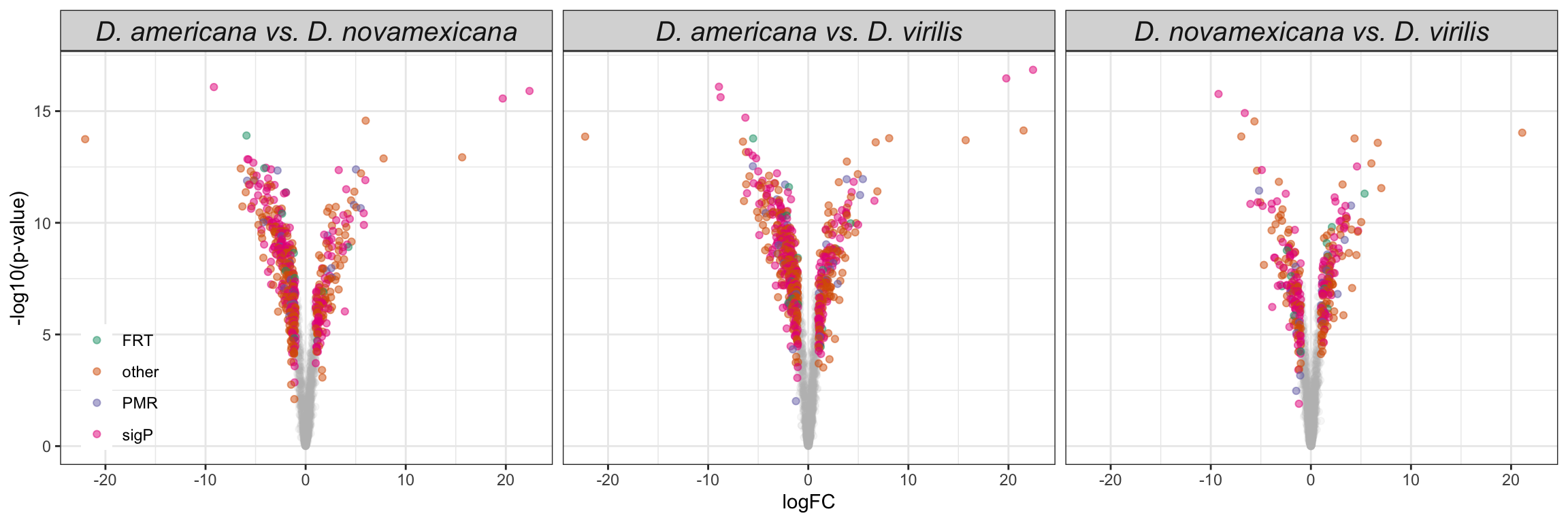
Are signal peps more likely to be DA?
# are signal peps more likely to be DA?
fem_TABLES %>%
  group_by(comparison, threshold, sigP) %>% dplyr::count() %>%
  ggplot(aes(x = threshold, y = n, fill = sigP)) +
  geom_col(position = 'fill') +
  facet_wrap(~comparison, nrow = 1,
             labeller = as_labeller(c(aVn = "D. americana vs. D. novamexicana",
                                      aVv = 'D. americana vs. D. virilis',
                                      nVv = "D. novamexicana vs. D. virilis"))) +
  theme_bw() +
  NULL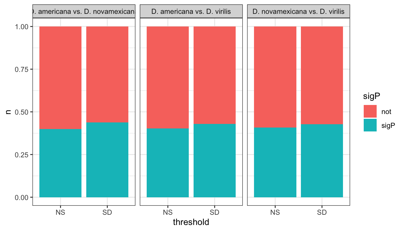
# Fisher's exact tests
fem_TABLES %>% group_by(comparison) %>%
  do(fit = broom::glance(fisher.test(as.matrix(xtabs(~ threshold + sigP, ., sparse = TRUE))))) %>%
  unnest(fit) %>%
  mutate(across(2:5, ~ round(.x, 2)),
         p.value = ifelse(p.value < 0.001, '< 0.001', round(p.value, 3)),
         comparison = recode(comparison,
                             aVn = "D. ame vs. D. nov", aVv = "D. ame vs. D. vir", nVv = 'D. nov vs. D. vir'),
         Estimate = paste0(estimate, ' (', conf.low, '-', conf.high, ')')) %>%
  dplyr::select(comparison, Estimate, p.value) %>%
  kable(caption = 'Proportion of signal peptides showing differential abundance between species. Fisher\'s exact tests') %>%
kable_styling(full_width = FALSE)| comparison | Estimate | p.value |
|---|---|---|
| D. ame vs. D. nov | 1.17 (0.96-1.43) | 0.10 |
| D. ame vs. D. vir | 1.12 (0.92-1.36) | 0.24 |
| D. nov vs. D. vir | 1.08 (0.86-1.36) | 0.49 |
# #save proteins minus ejaculate candidates i.e. remaining proteins as 'female'
# fem_TABLES %>%
#   filter(!genes %in% c(comb_TABLES %>% filter(adj.P.Val < 0.05  & logFC > 1) %>% pull(genes))) %>%
#   distinct(FBgn, .keep_all = TRUE) %>%
#   write_csv('output/ClueGOlists/TPP_all_NOTejac_FBgn.csv')
#
# #save proteins minus ejaculate candidates i.e. remaining proteins as 'female' & signal pep
# fem_TABLES %>%
#   filter(!genes %in% c(comb_TABLES %>% filter(adj.P.Val < 0.05  & logFC > 1) %>% pull(genes))) %>%
#   filter(sigP == 'sigP') %>%
#   distinct(FBgn, .keep_all = TRUE) %>%
#   write_csv('output/ClueGOlists/TPP_all_frtSigP_FBgn.csv')
#
# #save differentially abundant proteins to table for ClueGO
# fem_TABLES %>%
#   filter(!genes %in% c(comb_TABLES %>% filter(adj.P.Val < 0.05  & logFC > 1) %>% pull(genes)),
#          threshold == 'SD') %>%
#   distinct(FBgn, .keep_all = TRUE) %>%
#   write_csv('output/ClueGOlists/TPP_virgin_DA_multiDB.csv')
Heatmap
All proteins
fem_md <- data.frame(dgeFEMvoom$genes,
                     dgeFEMvoom$E) %>%
  rowwise() %>%
  mutate(`D. ame` = median(c(!!! rlang::syms(grep('A', names(.), value = TRUE)))),
         `D. nov` = median(c(!!! rlang::syms(grep('NV', names(.), value = TRUE)))),
         `D. vir` = median(c(!!! rlang::syms(grep('VV', names(.), value = TRUE))))) %>%
  left_join(vir_fbgn %>% select(-FBtr), by = c('genes' = 'gene_id')) %>%
  mutate(category = case_when(FBgn %in% sperm_mel$FBgn_v ~ 'sperm',
                              FBgn %in% wigbySFP$FBgn ~ 'Sfp',
                              TRUE ~ as.character(NA)),
         fem_cat = case_when(FBgn %in% STEP$FBgn ~ 'STEP',
                             FBgn %in% FRTbiased$FBgn_ID ~ 'FRT',
                             FBgn %in% virilisPMDE$FBgn_ID ~ 'pmr',
                             genes %in% vir_sig$protein ~ 'sig',
                             TRUE ~ as.character(NA))) %>%
  left_join(flybase_GO %>% dplyr::select(FBgn, Symbol = mel_GeneSymbol), by = 'FBgn') %>%
  mutate(Symbol = if_else(is.na(Symbol), FBgn, Symbol)) %>%
  distinct(genes, .keep_all = TRUE)

# scale data
mat_scaled_frt <- as.matrix(pheatmap:::scale_rows(fem_md[, 9:11]))

# # Dissimilarity matrix
df <- dist(mat_scaled_frt, method = "euclidean")
# # Hierarchical clustering using Complete Linkage
hc1f <- hclust(df, method = "complete" )

# Plot the dendrogram
#plot(hc1, cex = 0.6, hang = -1)

fviz_nbclust(mat_scaled_frt, FUN = hcut, method = "silhouette")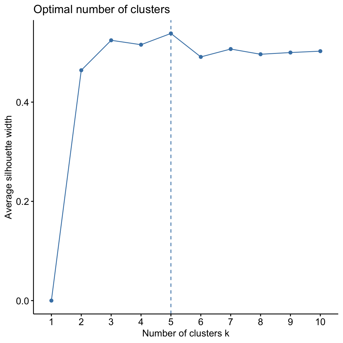
# Cut tree into 4 groups
sub_grpf <- cutree(hc1f, k = 5)

# Number of members in each cluster
#table(sub_grpf)

cat_labf <- rowAnnotation(clust_lab = sub_grpf,
                          col = list(clust_lab = setNames(cbPalette[2:(max(sub_grpf) + 1)], unique(sub_grpf))),
                          title = NULL,
                          show_annotation_name = FALSE)

frt_lab <- rowAnnotation(Category = fem_md$fem_cat,
                         col = list(Category = setNames(c('yellow', 'cyan', 'hotpink', 'red'),
                                                        unique(na.omit(fem_md$fem_cat)))),
                         frt_labs = anno_mark(at = c(grep('STEP', x = fem_md$fem_cat)),
                                              labels = na.omit(fem_md$Symbol[fem_md$fem_cat == 'STEP']),
                                              labels_gp = gpar(fontsize = 8)),
                         title = NULL,
                         na_col = NA,
                         show_annotation_name = FALSE)

frtha <- HeatmapAnnotation(species = anno_block(gp = gpar(fill = c(v.pal[c(3, 2, 1)])),
                                                labels = c(expression(italic('D. ame')),
                                                           expression(italic('D. nov')),
                                                           expression(italic('D. vir'))),
                                                labels_gp = gpar(col = c('white', 'white', 'black'),
                                                                 fontsize = 10)))

#pdf('plots/TPP_results/TPP_frt_compheatmap.pdf', height = 8, width = 5)
Heatmap(mat_scaled_frt,
        col = viridis::inferno(50),
        heatmap_legend_param = list(title = "log2(intensities)",
                                    #title_position = "leftcenter-rot",
                                    direction = "horizontal",
                                    at = c(-1.5, 0, 1.5)),
        right_annotation = frt_lab,
        left_annotation = cat_labf,
        top_annotation = frtha,
        show_row_names = FALSE,
        show_column_names = FALSE,
        row_split = max(sub_grpf),
        column_split = 3,
        column_gap = unit(0, "mm"),
        row_title = NULL,
        column_title = NULL)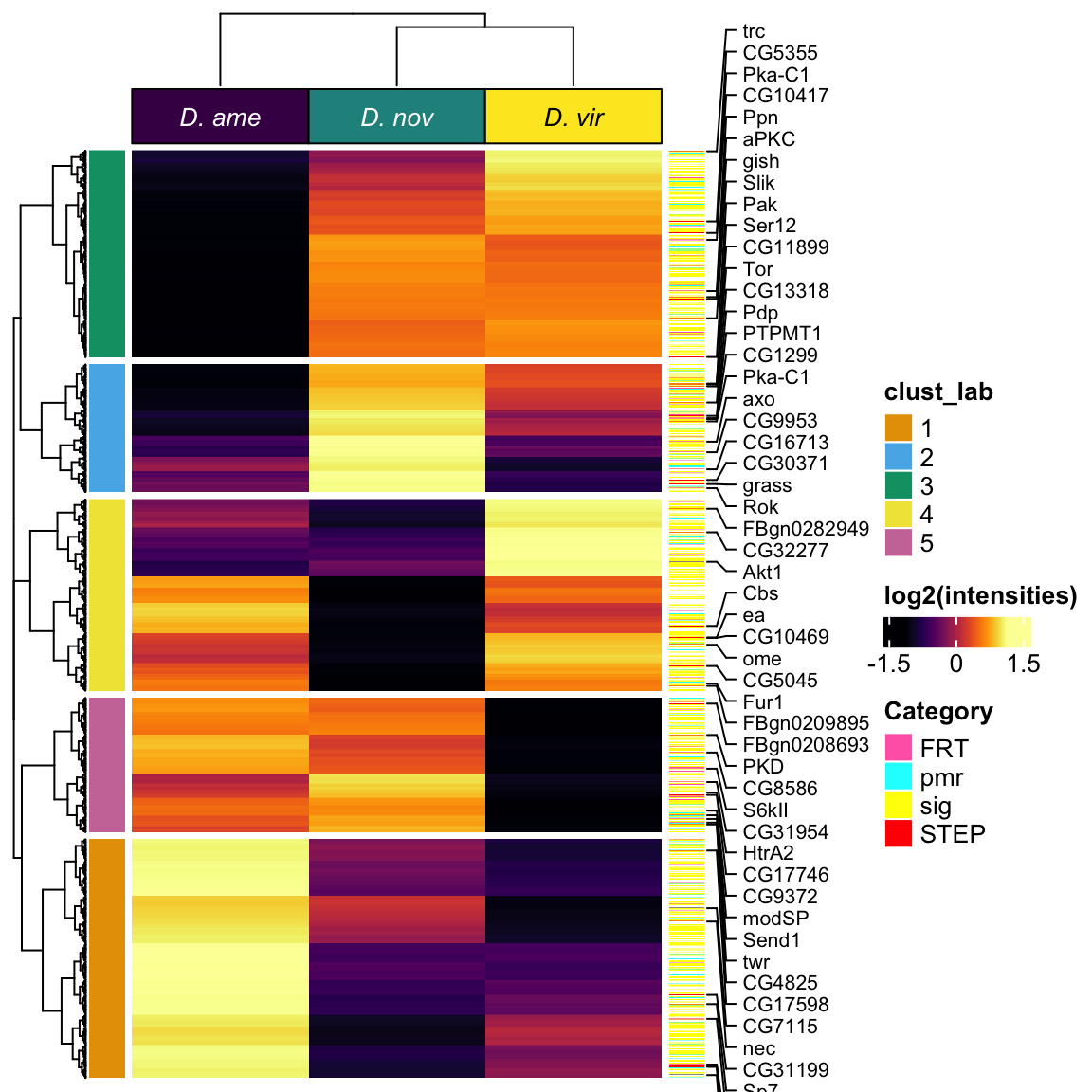
#dev.off()

y2 <- fem_md %>%
  bind_cols(cluster = sub_grpf) %>%
  dplyr::select(genes, FBgn, 9:11, cluster) %>%
  pivot_longer(cols = 3:5) %>%
  mutate(species = str_sub(name, 4, 4))

y2 %>%
  ggplot(aes(x = name, y = value, fill = name)) +
  geom_boxplot() +
  labs(x = 'Species') +
  scale_fill_viridis_d() +
  facet_wrap(~cluster) +
  ggpubr::stat_compare_means(aes(label = ..p.signif..),
                             comparisons = list(c('D. ame', 'D. nov'),
                                                c('D. ame', 'D. vir'),
                                                c('D. nov', 'D. vir')),
                             method = 't.test') +
  theme_bw() +
  theme(legend.position = '',
        axis.text.x = element_text(face = 'italic')) +
  NULL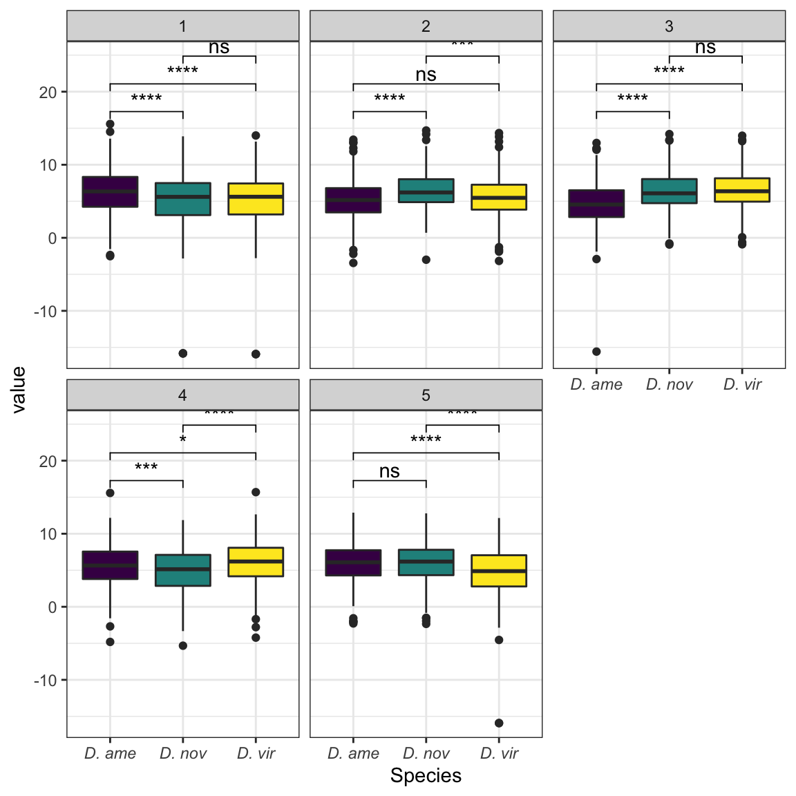
# Model fits
y2 %>% group_by(cluster) %>%
  do(fit = broom::glance(lm(value ~ name, data = .))) %>%
  unnest(fit) %>%
  mutate(p.value = ifelse(p.value < 0.001, '< 0.001', round(p.value, 3))) %>%
  dplyr::select(-adj.r.squared, -sigma, -c(df:df.residual)) %>%
  kable(digits = 3,
        caption = 'Model fits') %>%
kable_styling(full_width = FALSE)| cluster | r.squared | statistic | p.value | nobs |
|---|---|---|---|---|
| 1 | 0.018 | 14.383 | < 0.001 | 1554 |
| 2 | 0.031 | 13.262 | < 0.001 | 831 |
| 3 | 0.089 | 65.843 | < 0.001 | 1344 |
| 4 | 0.028 | 17.877 | < 0.001 | 1245 |
| 5 | 0.044 | 19.960 | < 0.001 | 873 |
# y2 %>% group_by(cluster) %>%
#   do(fit = broom::tidy(lm(value ~ name, data = .))) %>%
#   unnest(fit) %>%
#   mutate(p.value = ifelse(p.value < 0.001, '< 0.001', round(p.value, 3)),
#          sigLabel = case_when(p.value < 0.001 ~ "***",
#                               p.value < 0.01 ~ "**",
#                               p.value < 0.05 ~ "*",
#                               TRUE ~ '')) %>%
#   kable(digits = 3,
#         caption = 'Model estimates') %>%
#   kable_styling(full_width = FALSE)

plyr::ldply(lapply(split(y2, y2$cluster, drop = TRUE), function(x)
  {broom::tidy(TukeyHSD(aov(value ~ name, data = x)))})) %>%
  mutate(cluster = recode(.id,
                          `D. nov-D. ame` = "D. ame vs. D. nov",
                          `D. vir-D. ame` = "D. ame vs. D. vir",
                          `D. vir-D. nov` = 'D. nov vs. D. vir'),
         across(4:7, ~ round(.x, 2)),
         Estimate = paste0(estimate, ' (', conf.low, '-', conf.high, ')'),
         p.val = ifelse(adj.p.value < 0.001, "< 0.001", round(adj.p.value, 3)),
         sigLabel = case_when(adj.p.value < 0.001 ~ "***",
                              adj.p.value < 0.01 ~ "**",
                              adj.p.value < 0.05 ~ "*",
                              TRUE ~ '')) %>%
  dplyr::select(cluster, contrast, estimate, p.val, ` ` = sigLabel) %>%
  kable(digits = 3,
        caption = 'Post-hoc Tukey tests corrected for multiple testing') %>%
  kable_styling(full_width = FALSE) %>%
  group_rows("Cluster 1", 1, 3) %>%
  group_rows("Cluster 2 ", 4, 6) %>%
  group_rows("Cluster 3", 7, 9) %>%
group_rows("Cluster 4", 10, 12)| cluster | contrast | estimate | p.val | |
|---|---|---|---|---|
| Cluster 1 | ||||
| 1 | D. nov-D. ame | -0.95 | < 0.001 | *** |
| 1 | D. vir-D. ame | -0.97 | < 0.001 | *** |
| 1 | D. vir-D. nov | -0.02 | 0.993 | |
| Cluster 2 | ||||
| 2 | D. nov-D. ame | 1.20 | < 0.001 | *** |
| 2 | D. vir-D. ame | 0.40 | 0.21 | |
| 2 | D. vir-D. nov | -0.80 | 0.002 | ** |
| Cluster 3 | ||||
| 3 | D. nov-D. ame | 1.64 | < 0.001 | *** |
| 3 | D. vir-D. ame | 1.81 | < 0.001 | *** |
| 3 | D. vir-D. nov | 0.17 | 0.609 | |
| Cluster 4 | ||||
| 4 | D. nov-D. ame | -0.72 | 0.001 | ** |
| 4 | D. vir-D. ame | 0.49 | 0.044 |
|
| 4 | D. vir-D. nov | 1.21 | < 0.001 | *** |
| 5 | D. nov-D. ame | 0.08 | 0.946 | |
| 5 | D. vir-D. ame | -1.32 | < 0.001 | *** |
| 5 | D. vir-D. nov | -1.39 | < 0.001 | *** |
#### Differentially abundant proteins only
# fem_da <- fem_md %>% filter(genes %in% unique(fem_TABLES %>% filter(threshold != 'NS') %>% pull(genes)))
#
# # scale data
# mat_scaled_frt2 <- pheatmap:::scale_rows(fem_da[, 9:11])
#
# cat_labf2 <- rowAnnotation(Cluster = sub_grpf,
#                            col = list(Cluster = setNames(cbPalette[2:(max(sub_grpf) + 1)], unique(sub_grpf2))),
#                            title = NULL,
#                            show_annotation_name = FALSE)
#
# frt_lab <- rowAnnotation(Category = fem_da$fem_cat,
#                          col = list(Category = setNames(c('chocolate', 'orange', 'hotpink', 'cyan'),
#                                                         na.omit(unique(fem_da$fem_cat)))),
#                          frt_labs = anno_mark(at = c(grep('STEP', x = fem_da$fem_cat)),
#                                               labels = na.omit(fem_da$Symbol[fem_da$fem_cat == 'STEP']),
#                                               labels_gp = gpar(fontsize = 8)),
#                          title = NULL,
#                          na_col = NA,
#                          show_annotation_name = FALSE)
#
# #pdf('plots/frt_compheatmap_da.pdf', height = 8, width = 5)
# Heatmap(mat_scaled_frt2,
#         col = viridis::inferno(100),
#         heatmap_legend_param = list(title = "log2(intensities)",
#                                     title_position = "leftcenter-rot"),
#         right_annotation = frt_lab,
#         left_annotation = cat_labf2,
#         top_annotation = haha,
#         show_row_names = FALSE,
#         show_column_names = FALSE,
#         row_split = max(sub_grpf),
#         column_split = 3,
#         column_gap = unit(0, "mm"),
#         row_title = NULL,
#         column_title = NULL)
# #dev.off()

# y3 <- fem_da %>%
#   bind_cols(cluster = sub_grpf2) %>%
#   dplyr::select(genes, FBgn, 9:11, cluster) %>%
#   pivot_longer(cols = 3:5) %>%
#   mutate(species = str_sub(name, 4, 4))
#
# y3 %>%
#   ggplot(aes(x = factor(name, levels = c('D. vir', 'D. ame', 'D. nov')), y = value, fill = name)) +
#   geom_boxplot() +
#   labs(x = 'Species') +
#   scale_fill_viridis_d() +
#   facet_wrap(~cluster) +
#   ggsignif::geom_signif(comparisons = list(c("D. ame", "D. nov"),
#                                            c("D. ame", "D. vir"),
#                                            c("D. nov", "D. vir")),
#                         map_signif_level = TRUE) +
#   #coord_cartesian(ylim = c(2, 20)) +
#   theme_bw() +
#   theme(legend.position = '',
#         axis.text.x = element_text(face = 'italic')) +
#   NULL
#
# y3 %>%
#   mutate(cluster = paste('Cluster', cluster, sep = ' ')) %>%
#   ggplot(aes(x = factor(name, levels = c('D. vir', 'D. ame', 'D. nov')), y = value, fill = name)) +
#   gghalves::geom_half_point(aes(colour = name)) +
#   gghalves::geom_half_violin(aes(fill = name)) +
#   stat_pointinterval(pch = 21, fill = 'white') +
#   labs(x = 'Species', y = 'normalised abundance') +
#   scale_fill_viridis_d() +
#   scale_colour_viridis_d() +
#   facet_wrap(~cluster, scales = 'free_y') +
#   theme_bw() +
#   theme(legend.position = '',
#         axis.text.x = element_text(face = 'italic')) +
#   ggpubr::stat_compare_means(aes(label = ..p.signif..),
#                              comparisons = list(c('D. ame', 'D. nov'),
#                                                 c('D. ame', 'D. vir'),
#                                                 c('D. nov', 'D. vir')),
#                              method = 't.test') +
#   #ggsave('plots/frt_pointinterval.pdf', height = 6, width = 6, dpi = 600, useDingbats = FALSE) +
#   NULL
#
# # model fits
# y3 %>% group_by(cluster) %>%
#   do(fit = broom::tidy(lm(value ~ name, data = .))) %>%
#   unnest(fit) %>%
#   mutate(p.value = ifelse(p.value < 0.001, '< 0.001', round(p.value, 3)),
#          sigLabel = case_when(p.value < 0.001 ~ "***",
#                               p.value < 0.01 ~ "**",
#                               p.value < 0.05 ~ "*",
#                               TRUE ~ '')) %>%
#   kable(digits = 3,
#         caption = 'Model estimates') %>%
#   kable_styling(full_width = FALSE)
#
# # posthoc tests
# plyr::ldply(lapply(split(y3, y3$cluster, drop = T), function(x)
#   {broom::tidy(TukeyHSD(aov(value ~ name, data = x)))})) %>%
#   mutate(cluster = recode(.id,
#                       `D. nov-D. ame` = "D. ame vs. D. nov",
#                       `D. vir-D. ame` = "D. ame vs. D. vir",
#                       `D. vir-D. nov` = 'D. nov vs. D. vir'),
#          across(4:7, ~ round(.x, 2)),
#          Estimate = paste0(estimate, ' (', conf.low, '-', conf.high, ')'),
#          p.val = ifelse(adj.p.value < 0.001, "< 0.001", round(adj.p.value, 3)),
#          sigLabel = case_when(adj.p.value < 0.001 ~ "***",
#                               adj.p.value < 0.01 ~ "**",
#                               adj.p.value < 0.05 ~ "*",
#                               TRUE ~ '')) %>%
#   dplyr::select(contrast, Estimate, p.val, ` ` = sigLabel) %>%
#   kable(digits = 3,
#         caption = 'Post-hoc Tukey tests corrected for multiple testing') %>%
#   kable_styling(full_width = FALSE) %>%
#   group_rows("Cluster 1", 1, 3) %>%
#   group_rows("Cluster 2 ", 4, 6) %>%
#   group_rows("Cluster 3", 7, 9) %>%
#   group_rows("Cluster 4", 10, 12)
Duplicated genes
All duplicate data
multiDB %>%
  filter(Orthogroup %in% unique(mdb2[which(duplicated(mdb2$Orthogroup) == TRUE), "Orthogroup"])$Orthogroup)
# A tibble: 669 × 18
protein_vir Orthogroup AM1 AM2 AM3 AV1 AV2 NM1 NM2
<chr> <chr> <dbl> <dbl> <dbl> <dbl> <dbl> <dbl> <dbl>
1 MSTRG.7265 OG0001115 130615. 148100. 105415. 1.54e5 1.44e5 2.13e6 2.61e6
2 MSTRG.11558 OG0000593 181828. 208559. 165115. 2.20e5 2.29e5 2.13e5 1.90e5
3 MSTRG.3484 OG0000593 181828. 208559. 165115. 2.20e5 2.29e5 2.13e5 1.90e5
4 MSTRG.11574 OG0000594 570837. 418525. 508847. 6.20e5 7.62e5 3.69e6 3.86e6
5 MSTRG.11574 OG0000594 206081. 147123. 158241. 2.35e5 2.35e5 3.69e6 3.86e6
6 MSTRG.11618 OG0000312 1176062. 834103 1065069. 1.35e6 1.50e6 2.13e6 2.43e6
7 MSTRG.11629 OG0000312 1176062. 834103 1065069. 1.35e6 1.50e6 2.13e6 2.43e6
8 MSTRG.11618 OG0000312 2143772. 1408941. 2207962. 2.10e6 2.88e6 2.13e6 2.43e6
9 MSTRG.11629 OG0000312 2143772. 1408941. 2207962. 2.10e6 2.88e6 2.13e6 2.43e6
10 MSTRG.11709 OG0000174 175350. 110755. 167556. 1.91e5 2.08e5 1.25e5 1.47e5
# … with 659 more rows, and 9 more variables: NM3 <dbl>, NV1 <dbl>, NV2 <dbl>,
# VM1 <dbl>, VM2 <dbl>, VM3 <dbl>, VV1 <dbl>, VV2 <dbl>, VV3 <dbl>Mated vs. virgin
# duplicated genes
comb_TABLES_dup <- comb_TABLES %>% filter(Orthogroup %in% ortho_dups$Orthogroup)

comb_TABLES_dup %>%
  ggplot(aes(x = logFC, y = -log10(P.Value), colour = DA)) +
  geom_point(alpha = .6) +
  scale_colour_manual(values = cbPalette[4:1]) +
  labs(y = '-log10(p-value)') +
  facet_wrap(~species) +
  theme_bw()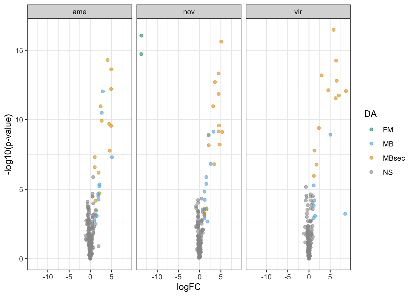
n_distinct(comb_TABLES_dup$genes)[1] 185Divergence between species - ejaculate candidates
# duplicated genes
mated_TABLES_dup <- mated_TABLES %>% filter(Orthogroup %in% ortho_dups$Orthogroup)

mated_TABLES_dup %>%
  ggplot(aes(x = logFC, y = -log10(P.Value))) +
  geom_point(data = . %>% filter(threshold == 'NS'), alpha = .75, colour = 'grey') +
  geom_point(data = . %>% filter(threshold != 'NS'), aes(colour = DA), alpha = .5) +
  scale_colour_manual(values = cbPalette[4:1]) +
  labs(y = '-log10(p-value)') +
  facet_wrap(~comparison) +
  theme_bw()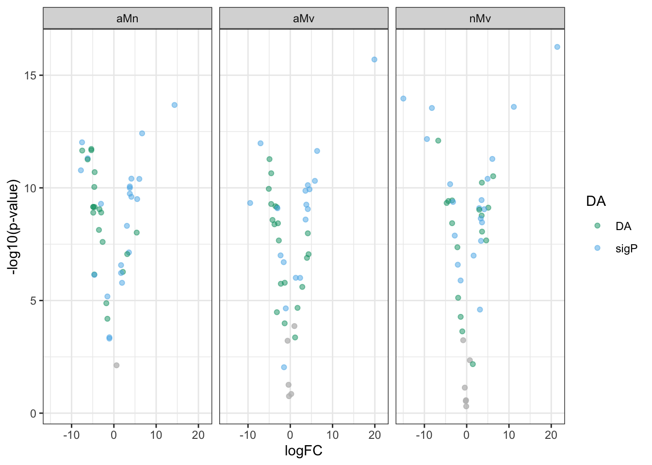
mated_TABLES_dup %>%
  group_by(Orthogroup, comparison) %>%
  summarise(N = n(),
            mnlfc = mean(logFC),
            mnexp = mean(AveExpr),
            sdlfc = sd(logFC)) %>%
  dplyr::mutate(sdlfc = replace_na(sdlfc, 1)) %>%
  ggplot(aes(x = mnexp, y = mnlfc)) +
  geom_point(aes(colour = N,  size = sdlfc)) +
  facet_wrap(~comparison) +
  scale_colour_viridis_c() +
  theme_bw() +
  theme() +
  NULL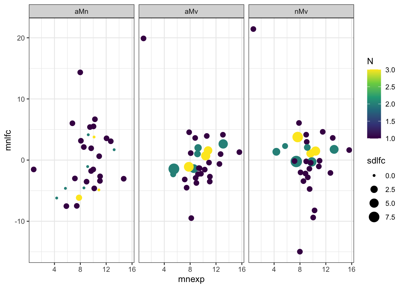
# differentially abundant duplicates
da_dup <- mated_TABLES_dup %>% filter(threshold == 'SD')

upset(fromList(list(aVn = split(da_dup, da_dup$comparison)[[1]][[1]],
                    aVv = split(da_dup, da_dup$comparison)[[2]][[1]],
                    nVv = split(da_dup, da_dup$comparison)[[3]][[1]])))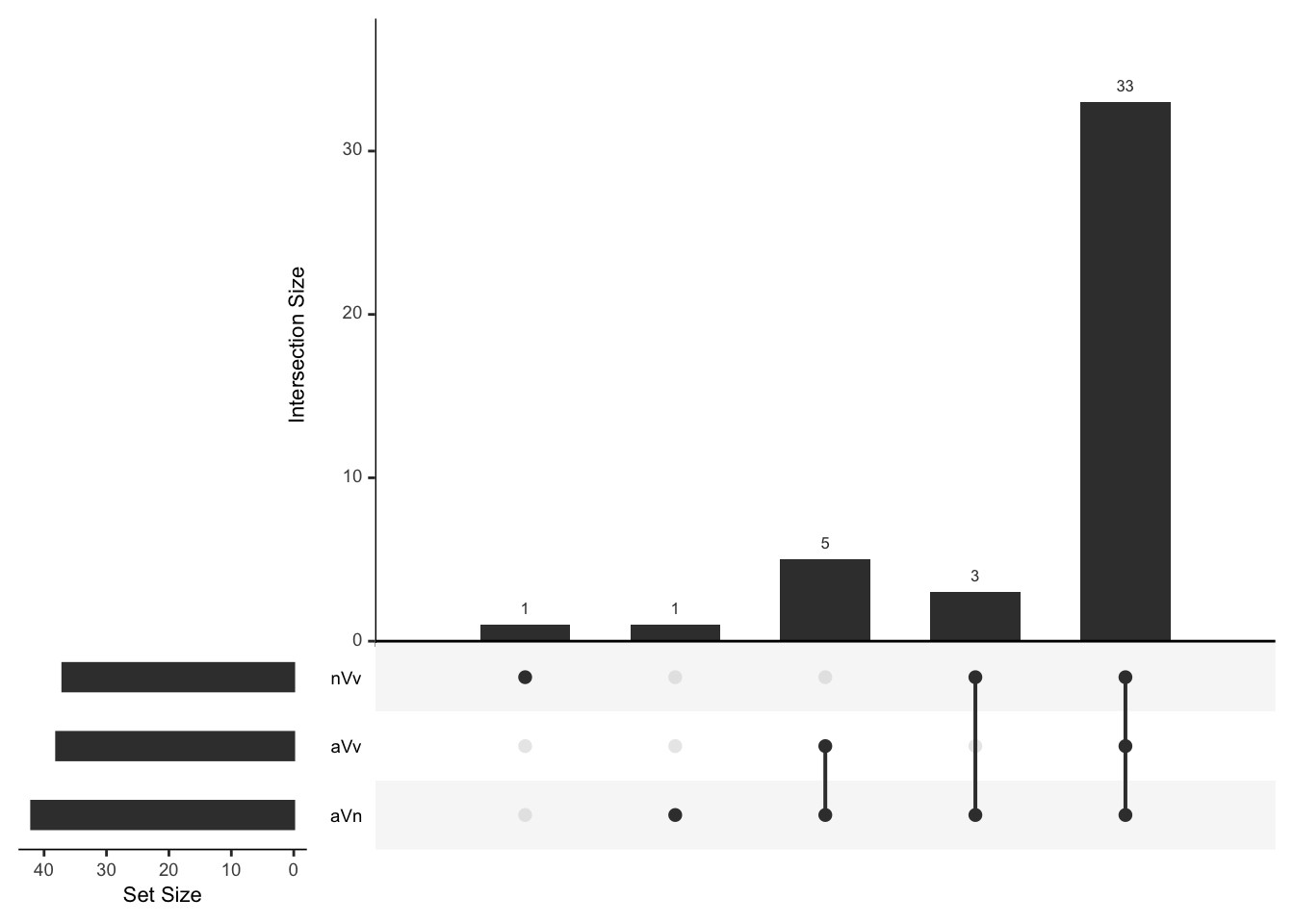
#
sfp_dup_dat <- data.frame(dgeSFPvoom$genes,
                          dgeSFPvoom$E) %>%
  rowwise() %>%
  mutate(`D. ame` = median(c(!!! rlang::syms(grep('AM', names(.), value = TRUE)))),
         `D. nov` = median(c(!!! rlang::syms(grep('NM', names(.), value = TRUE)))),
         `D. vir` = median(c(!!! rlang::syms(grep('VM', names(.), value = TRUE))))) %>%
  left_join(vir_fbgn %>% select(-FBtr), by = c('genes' = 'gene_id')) %>%
  filter(Orthogroup %in% ortho_dups$Orthogroup) %>%
  arrange(Orthogroup) %>%
  mutate(da = if_else(Orthogroup %in% da_dup$Orthogroup, "sd", "ns"))

sfp_dup_md <- sfp_dup_dat %>% select(`D. ame`, `D. nov`, `D. vir`,
                                     Orthogroup, da)

sf_dup_scaled <- as.matrix(pheatmap:::scale_rows(sfp_dup_md[, 1:3]))

# heatmap annotations
left_lab <- rowAnnotation(Orthogroup = sfp_dup_dat$Orthogroup,
                          col = list(Orthogroup = setNames(rainbow(n_distinct(sfp_dup_dat$Orthogroup)),
                                                           unique(sfp_dup_dat$Orthogroup))),
                          title = NULL,
                          show_annotation_name = FALSE,
                          show_legend = FALSE)

right_lab <- rowAnnotation(Category = sfp_dup_md$da,
                           col = list(Category = c(sd = "red",
                                                   ns = NA)),
                           title = NULL,
                           show_annotation_name = FALSE)

Heatmap(sf_dup_scaled,
        col = viridis::inferno(25),
        heatmap_legend_param = list(title = "log2(intensities)",
                                    #title_position = "leftcenter-rot",
                                    direction = "horizontal",
                                    at = c(-1.5, 0, 1.5)),
        #right_annotation = right_lab,
        left_annotation = left_lab,
        top_annotation = sfpha,
        show_row_names = FALSE,
        cluster_rows = FALSE,
        #show_column_names = FALSE,
        #row_split = max(sub_grp),
        column_split = 3,
        column_gap = unit(0, "mm"),
        row_title = NULL,
        column_title = NULL)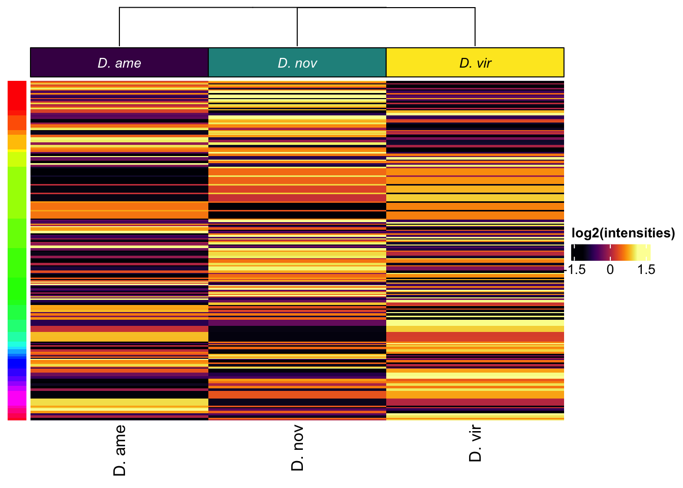
sfp_dup_dat %>%
  pivot_longer(cols = 11:13) %>%
  distinct(Orthogroup, genes, name, value) %>%
  #mutate(species = str_sub(name, 1, 1)) %>%
  ggplot(aes(name, y = value, colour = genes)) +
  geom_line(aes(group = Orthogroup), position = position_dodge(width = .25)) +
  geom_jitter(position = position_jitterdodge(dodge.width = .5, jitter.width = .25), alpha = .5) +
  facet_wrap(~ Orthogroup, scales = "free_y") +
  scale_colour_viridis_d() +
  theme_bw() +
  theme(legend.position = '') +
  NULL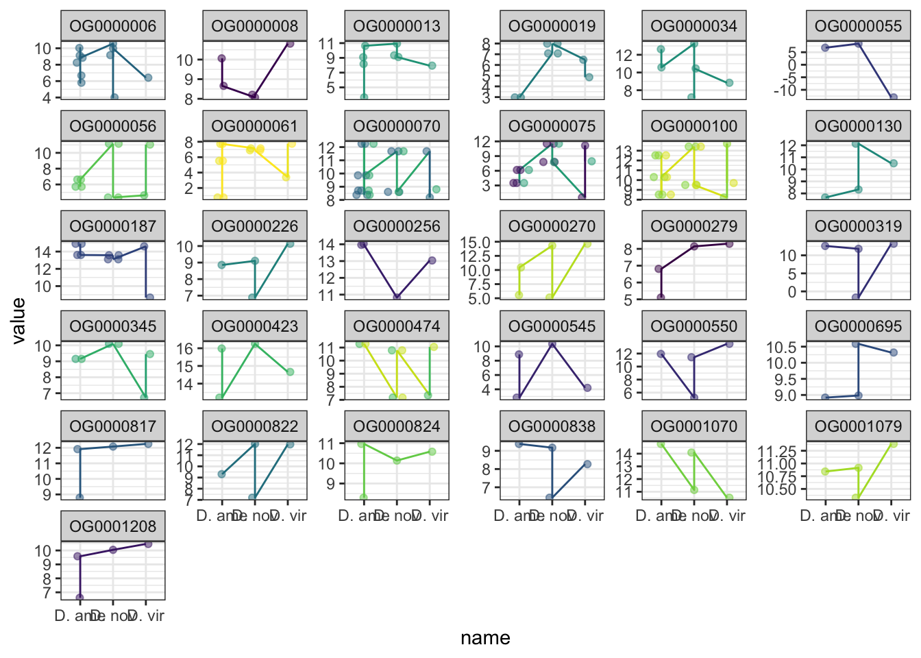
sfp_dup_dat %>% filter(Orthogroup %in% da_dup$Orthogroup) %>%
  mutate(da_pattern = case_when(`D. ame` > `D. nov` & `D. ame` > `D. vir` ~ "ame_up",
                                `D. ame` < `D. nov` & `D. nov` > `D. vir` ~ "nov_up",
                                `D. ame` < `D. vir` & `D. nov` < `D. vir` ~ "vir_up")) %>%
  pivot_longer(cols = 11:13) %>%
  distinct(Orthogroup, genes, name, value, da_pattern) %>%
  group_by(Orthogroup, genes, name, da_pattern) %>%
  summarise(N = n(),
            #mnlfc = mean(logFC),
            mnexp = mean(value),
            sdexp = sd(value)) %>%
  ggplot(aes(name, y = mnexp)) +
  geom_line(aes(group = Orthogroup), alpha = .5) +
  geom_point(aes(size = N, fill = sdexp), shape = 21) +
  facet_wrap(~ da_pattern) +
  scale_colour_viridis_d(guide = "none") +
  scale_fill_viridis_c() +
  theme_bw() +
  #theme(legend.position = '') +
  NULL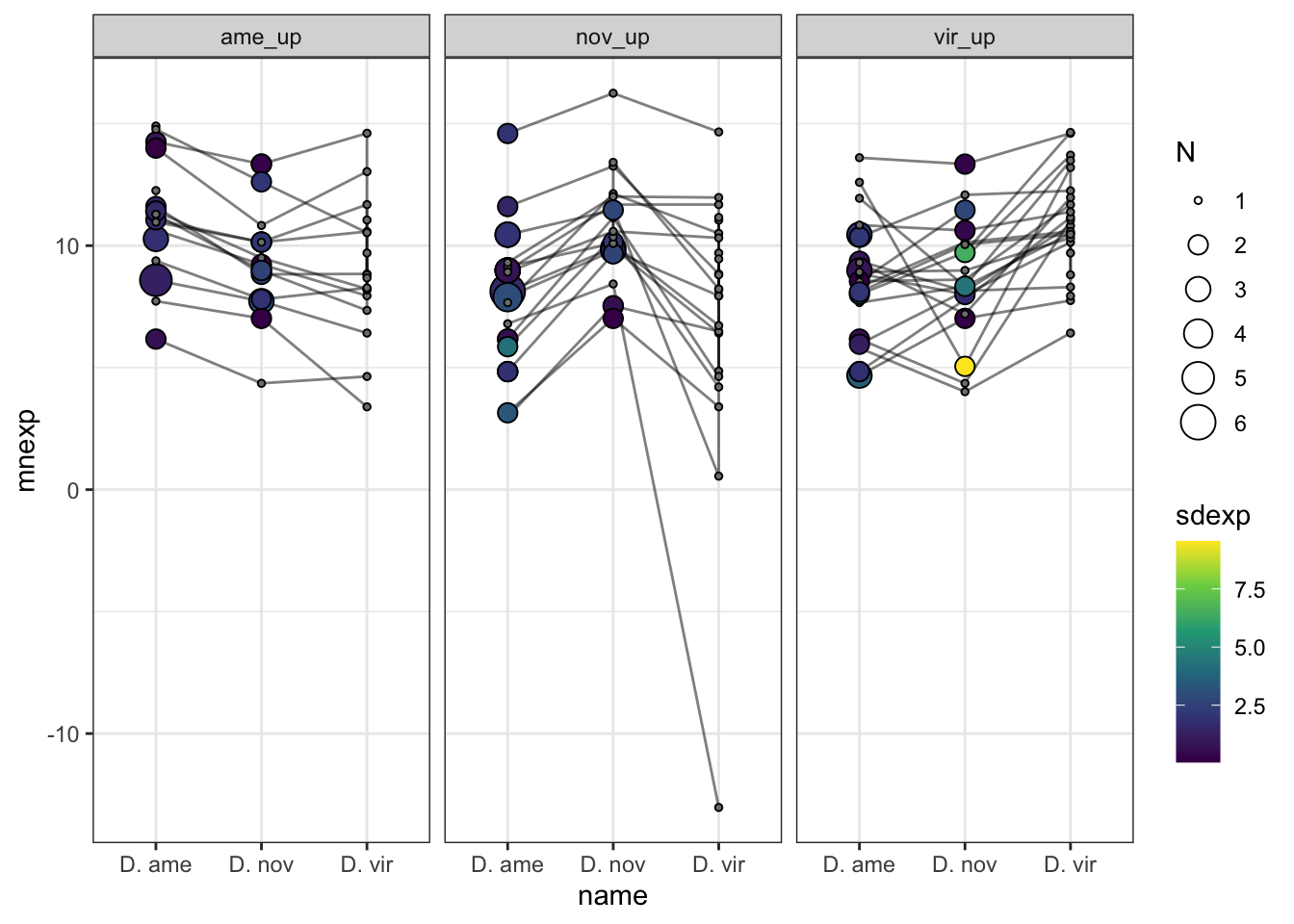
sfp_orths <- orthogroup_long %>%
  filter(Orthogroup %in% da_dup$Orthogroup)

sfp_orths %>% map_dbl(n_distinct)
Orthogroup species protein
31 3 255 da_dup %>% map_dbl(n_distinct) genes logFC AveExpr t P.Value adj.P.Val B
43 106 76 117 117 113 117
comparison threshold FBgn Orthogroup sigP sperm Sfp
3 1 43 31 2 2 2
DA
2 sfp_orths <- mdb_counts %>%
filter(Orthogroup %in% da_dup$Orthogroup)
# number of proteins belonging to an orthogroup - most proteins are single copy
sfp_orths %>%
group_by(name, value) %>%
count() %>%
ggplot(aes(x = factor(value), y = n, fill = name)) +
geom_bar(stat = "identity", position = "dodge") +
scale_fill_viridis_d()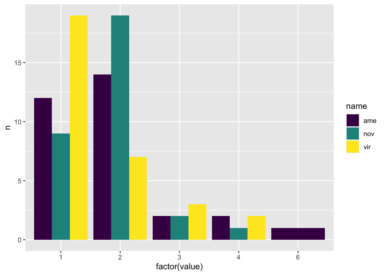
# proteins belonging to orthogroup/families
ame_dups_sfp <- ortho_ame %>% filter(Orthogroup %in% da_dup$Orthogroup) %>% drop_na(Orthogroup)
nov_dups_sfp <- ortho_nov %>% filter(Orthogroup %in% da_dup$Orthogroup) %>% drop_na(Orthogroup)
vir_dups_sfp <- ortho_vir %>% filter(Orthogroup %in% da_dup$Orthogroup) %>% drop_na(Orthogroup)

library(ggalluvial)
bind_rows(ame_dups_sfp %>% mutate(species = "Dame"),
          nov_dups_sfp %>% mutate(species = "Dnov"),
          vir_dups_sfp %>% mutate(species = "Dvir")) %>%
  group_by(species, Orthogroup) %>%
  count(name = "N") %>%
  group_by(species, N, Orthogroup) %>%
  count() %>%
  mutate(N = fct_reorder(as.character(N), as.integer(N))) %>%
  ggplot(aes(x = species, stratum = N, alluvium = Orthogroup,
           y = n, label = N)) +
  #geom_flow(aes(fill = N)) +
  geom_alluvium(aes(fill = N)) +
  geom_stratum(aes(fill = N), alpha = .05) +
  geom_text(stat = "stratum") +
  scale_fill_viridis_d() +
  theme_bw() +
  theme() +
  NULL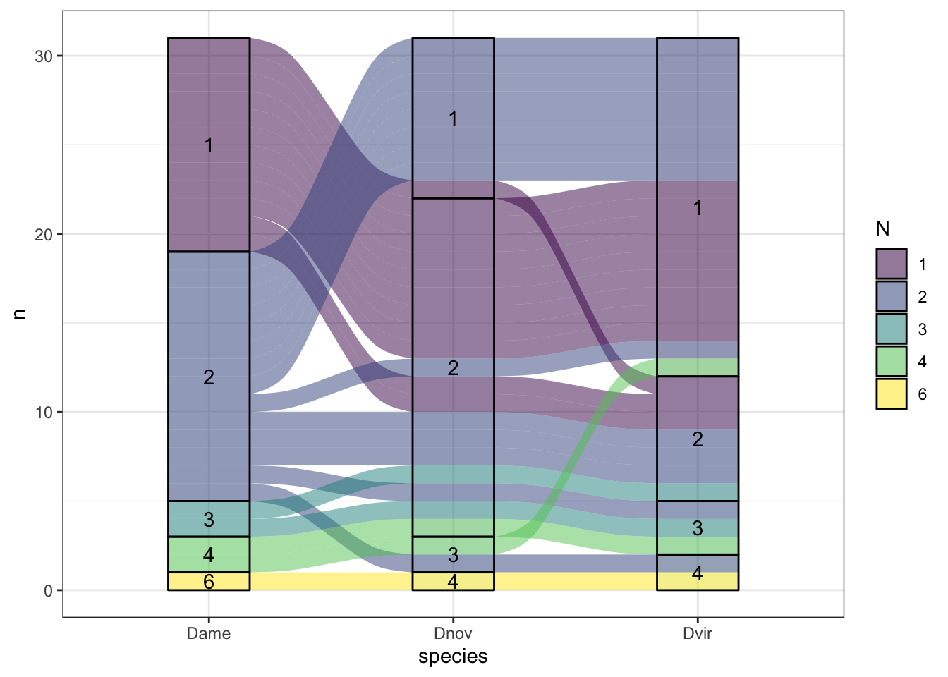
da_dup %>% #filter(Orthogroup == "OG0000006") %>%
  left_join(wigbySFP, by = 'FBgn') %>%
  drop_na(Symbol)
genes logFC AveExpr t P.Value adj.P.Val
1 MSTRG.11262 6.675042 10.257687 44.14013 3.807778e-13 7.635597e-12
2 MSTRG.9917 -6.205753 3.619289 -34.08147 5.472505e-12 7.446516e-11
3 MSTRG.382 3.771075 9.852041 26.04709 8.633707e-11 7.649866e-10
4 MSTRG.1594 3.771075 10.865206 25.65312 1.008983e-10 8.542719e-10
5 MSTRG.1928 3.771075 9.663222 24.22290 1.812961e-10 1.469656e-09
6 MSTRG.1928 4.153463 10.709003 26.37464 7.597581e-11 5.462109e-10
7 MSTRG.382 3.584724 10.897822 24.94417 1.343601e-10 8.676473e-10
8 MSTRG.1594 -3.033735 10.716738 -20.92741 8.034032e-10 4.193104e-09
9 MSTRG.9917 4.150120 5.892643 16.23410 1.040782e-08 3.776553e-08
10 MSTRG.11262 -1.556136 10.257687 -12.04629 1.987268e-07 5.221717e-07
11 MSTRG.11262 -8.231178 10.257687 -56.73319 2.847237e-14 4.172297e-13
12 MSTRG.1928 3.520604 9.514754 22.72051 3.482615e-10 2.948614e-09
13 MSTRG.1594 -3.223834 9.670957 -22.29797 4.216032e-10 3.250621e-09
14 MSTRG.382 2.951865 9.703573 20.94004 7.984970e-10 5.156396e-09
15 MSTRG.9917 3.540888 3.619289 19.44471 1.691895e-09 8.710971e-09
B comparison threshold FBgn Orthogroup sigP sperm Sfp DA
1 19.989191 aMn SD FBgn0206811 OG0000550 sigP not Sfp sigP
2 17.739527 aMn SD FBgn0207519 OG0000061 not not Sfp DA
3 15.445811 aMn SD FBgn0211755 OG0000070 sigP not Sfp sigP
4 15.295985 aMn SD FBgn0211069 OG0000070 sigP not Sfp sigP
5 14.727926 aMn SD FBgn0210521 OG0000070 sigP not Sfp sigP
6 15.560827 aMv SD FBgn0210521 OG0000070 sigP not Sfp sigP
7 15.019514 aMv SD FBgn0211755 OG0000070 sigP not Sfp sigP
8 13.255783 aMv SD FBgn0211069 OG0000070 sigP not Sfp sigP
9 10.695023 aMv SD FBgn0207519 OG0000061 not not Sfp DA
10 7.511216 aMv SD FBgn0206811 OG0000550 sigP not Sfp sigP
11 21.901959 nMv SD FBgn0206811 OG0000550 sigP not Sfp sigP
12 14.084740 nMv SD FBgn0210521 OG0000070 sigP not Sfp sigP
13 13.897513 nMv SD FBgn0211069 OG0000070 sigP not Sfp sigP
14 13.261334 nMv SD FBgn0211755 OG0000070 sigP not Sfp sigP
15 12.511509 nMv SD FBgn0207519 OG0000061 not not Sfp DA
FBgn_mel Symbol FBtr
1 FBgn0034417 CG15117 FBtr0434777
2 FBgn0050104 NT5E-2 FBtr0236304
3 FBgn0037889 scpr-A FBtr0240603
4 FBgn0037889 scpr-A FBtr0239907
5 FBgn0037889 scpr-A FBtr0239345
6 FBgn0037889 scpr-A FBtr0239345
7 FBgn0037889 scpr-A FBtr0240603
8 FBgn0037889 scpr-A FBtr0239907
9 FBgn0050104 NT5E-2 FBtr0236304
10 FBgn0034417 CG15117 FBtr0434777
11 FBgn0034417 CG15117 FBtr0434777
12 FBgn0037889 scpr-A FBtr0239345
13 FBgn0037889 scpr-A FBtr0239907
14 FBgn0037889 scpr-A FBtr0240603
15 FBgn0050104 NT5E-2 FBtr0236304da_dup %>% filter(Orthogroup == "OG0000070") genes logFC AveExpr t P.Value adj.P.Val B
1 MSTRG.382 3.771075 9.852041 26.04709 8.633707e-11 7.649866e-10 15.44581
2 MSTRG.1594 3.771075 10.865206 25.65312 1.008983e-10 8.542719e-10 15.29599
3 MSTRG.1928 3.771075 9.663222 24.22290 1.812961e-10 1.469656e-09 14.72793
4 MSTRG.1928 4.153463 10.709003 26.37464 7.597581e-11 5.462109e-10 15.56083
5 MSTRG.382 3.584724 10.897822 24.94417 1.343601e-10 8.676473e-10 15.01951
6 MSTRG.1594 -3.033735 10.716738 -20.92741 8.034032e-10 4.193104e-09 13.25578
7 MSTRG.1928 3.520604 9.514754 22.72051 3.482615e-10 2.948614e-09 14.08474
8 MSTRG.1594 -3.223834 9.670957 -22.29797 4.216032e-10 3.250621e-09 13.89751
9 MSTRG.382 2.951865 9.703573 20.94004 7.984970e-10 5.156396e-09 13.26133
comparison threshold FBgn Orthogroup sigP sperm Sfp DA
1 aMn SD FBgn0211755 OG0000070 sigP not Sfp sigP
2 aMn SD FBgn0211069 OG0000070 sigP not Sfp sigP
3 aMn SD FBgn0210521 OG0000070 sigP not Sfp sigP
4 aMv SD FBgn0210521 OG0000070 sigP not Sfp sigP
5 aMv SD FBgn0211755 OG0000070 sigP not Sfp sigP
6 aMv SD FBgn0211069 OG0000070 sigP not Sfp sigP
7 nMv SD FBgn0210521 OG0000070 sigP not Sfp sigP
8 nMv SD FBgn0211069 OG0000070 sigP not Sfp sigP
9 nMv SD FBgn0211755 OG0000070 sigP not Sfp sigPcircos
# library(circlize)
#
# sfp_dup_dat %>%
#   group_by(Orthogroup) %>% count()
#
#
# og_wide <- og_counts %>% filter(Orthogroup %in% multiDB$Orthogroup) %>%
#   filter(Orthogroup %in% sfp_dup_dat$Orthogroup) %>%
#   #pivot_wider(names_from = "species", values_from = orth_numb) %>%
#   pivot_wider(names_from = "species", values_from = Orthogroup)
#
#
# og_counts %>% filter(Orthogroup %in% sfp_dup_dat$Orthogroup) %>%
#   group_by(species, Orthogroup) %>% count() %>%
#   pivot_wider(names_from = "species", values_from = n)
#
# ass_counts <- og_wide %>%
#   mutate(#means = rowMeans(.[elected_cols], na.rm = T),
#          an_count_na = 2 - apply(.[c("Dame", "Dnov")], 1, function(x) sum(is.na(x))),
#          av_count_na = 2 - apply(.[c("Dame", "Dvir")], 1, function(x) sum(is.na(x))),
#          nv_count_na = 2 - apply(.[c("Dnov", "Dvir")], 1, function(x) sum(is.na(x))))
#
# df <- data.frame(from = rep(c("Dame", "Dame", "Dnov"), each = 66),
#                  to = rep(c("Dnov", "Dvir", "Dvir"), each = 66),
#                  value = c(ass_counts$an_count_na, ass_counts$av_count_na, ass_counts$nv_count_na))
#
# chordDiagram(df)
#
# df <- data.frame(from = c("Dame", "Dame", "Dnov"),
#                  to = c("Dnov", "Dvir", "Dvir"),
#                  value = c(sum(ass_counts$an_count_na == 2, na.rm = TRUE),
#                            sum(ass_counts$av_count_na == 2, na.rm = TRUE),
#                            sum(ass_counts$nv_count_na == 2, na.rm = TRUE)))
#
# chordDiagram(df)
#
# mat = matrix(1:9, 3)
# rownames(mat) = letters[1:3]
# colnames(mat) = LETTERS[1:3]
# mat
# chordDiagram(mat)
#
#
#
# # Initialize the plot.
# par(mar = c(1, 1, 1, 1) )
# circos.initialize(factors = data$factor, x = data$x )
#
# # Build the regions of track #1
# circos.trackPlotRegion(factors = data$factor, y=data$y , bg.col = rgb(0.1,0.1,seq(0,1,0.1),0.4) , bg.border = NA)
#
# # Add a link between a point and another
# circos.link("a", 0, "b", 0, h = 0.4)
#
# # Add a link between a point and a zone
# circos.link("e", 0, "g", c(-1,1), col = "green", lwd = 2, lty = 2, border="black" )
#
# # Add a link between a zone and another
# circos.link("c", c(-0.5, 0.5), "d", c(-0.5,0.5), col = "red", border = "blue", h = 0.2)
#
#
#
#
#
# circos.par("track.height" = 0.1)
# circos.initialize(og_counts$species, x = og_counts$orth_numb)
#
# circos.track(og_counts$species, y = og_counts$N,
#     panel.fun = function(x, y) {
#         circos.text(CELL_META$xcenter,
#             CELL_META$cell.ylim[2] + mm_y(5),
#             CELL_META$sector.index)
#         circos.axis(labels.cex = 0.6)
# })
#
# col = rep(c("#FF0000", "#00FF00"), 4)
# circos.trackPoints(og_counts$species, og_counts$orth_numb, og_counts$N, col = col, pch = 16, cex = 0.5)
# circos.text(-1, 0.5, "text", sector.index = "a", track.index = 1)
#
# bgcol = rep(c("#EFEFEF", "#CCCCCC"), 4)
# circos.trackHist(og_counts$species, og_counts$N, bin.size = 0.2, bg.col = bgcol, col = NA)
#
# circos.track(og_counts$species, og_counts$orth_numb, og_counts$N,
#     panel.fun = function(x, y) {
#         ind = sample(length(x), 10)
#         x2 = x[ind]
#         y2 = y[ind]
#         od = order(x2)
#         circos.lines(x2[od], y2[od])
# })
#
Divergence between species - FRT
# duplicated genes
fem_TABLES_dup <- fem_TABLES %>% filter(Orthogroup %in% ortho_dups$Orthogroup)

fem_TABLES_dup %>%
  ggplot(aes(x = logFC, y = -log10(P.Value))) +
  geom_point(data = . %>% filter(threshold == 'NS'), alpha = .5, colour = 'grey') +
  geom_point(data = . %>% filter(threshold != 'NS'), aes(colour = spec), alpha = .5) +
  scale_colour_manual(values = cbPalette[5:2]) +
  labs(y = '-log10(p-value)') +
  facet_wrap(~comparison) +
  theme_bw()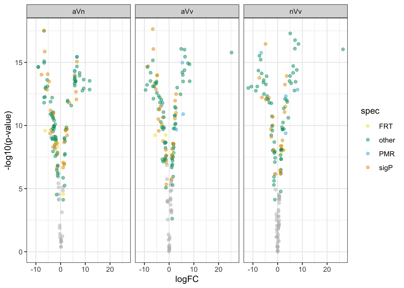
# differentially abundant duplicates
da_dup_fem <- fem_TABLES %>% filter(Orthogroup %in% ortho_dups$Orthogroup, threshold == 'SD')

upset(fromList(list(aVn = split(da_dup_fem, da_dup_fem$comparison)[[1]][[1]],
                    aVv = split(da_dup_fem, da_dup_fem$comparison)[[2]][[1]],
                    nVv = split(da_dup_fem, da_dup_fem$comparison)[[3]][[1]])))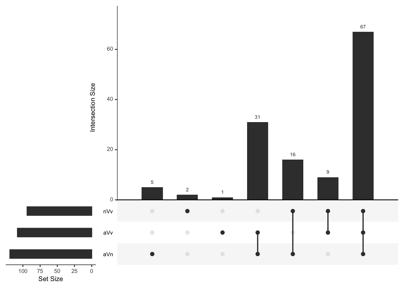
frt_dup_dat <- data.frame(dgeFEMvoom$genes,
                          dgeFEMvoom$E) %>%
  rowwise() %>%
  mutate(`D. ame` = median(c(!!! rlang::syms(grep('AV', names(.), value = TRUE)))),
         `D. nov` = median(c(!!! rlang::syms(grep('NV', names(.), value = TRUE)))),
         `D. vir` = median(c(!!! rlang::syms(grep('VV', names(.), value = TRUE))))) %>%
  left_join(vir_fbgn %>% select(-FBtr), by = c('genes' = 'gene_id')) %>%
  filter(Orthogroup %in% ortho_dups$Orthogroup) %>%
  arrange(Orthogroup) %>%
  mutate(da = if_else(Orthogroup %in% da_dup_fem$Orthogroup, "sd", "ns"))

frt_dup_md <- frt_dup_dat %>% select(`D. ame`, `D. nov`, `D. vir`, Orthogroup, da)

frt_dup_scaled <- as.matrix(pheatmap:::scale_rows(frt_dup_md[, 1:3]))

# heatmap annotations
left_labf <- rowAnnotation(Orthogroup = frt_dup_dat$Orthogroup,
                          col = list(Orthogroup = setNames(rainbow(n_distinct(frt_dup_dat$Orthogroup)),
                                                           unique(frt_dup_dat$Orthogroup))),
                          title = NULL,
                          show_annotation_name = FALSE,
                          show_legend = FALSE)

right_labf <- rowAnnotation(Category = frt_dup_md$da,
                           col = list(Category = c(sd = "red",
                                                   ns = NA)),
                           title = NULL,
                           show_annotation_name = FALSE)

Heatmap(frt_dup_scaled,
        col = viridis::inferno(50),
        heatmap_legend_param = list(title = "log2(intensities)",
                                    #title_position = "leftcenter-rot",
                                    direction = "horizontal",
                                    at = c(-1.5, 0, 1.5)),
        right_annotation = right_labf,
        left_annotation = left_labf,
        top_annotation = frtha,
        show_row_names = FALSE,
        cluster_rows = FALSE,
        #show_column_names = FALSE,
        #row_split = max(sub_grp),
        column_split = 3,
        column_gap = unit(0, "mm"),
        row_title = NULL,
        column_title = NULL)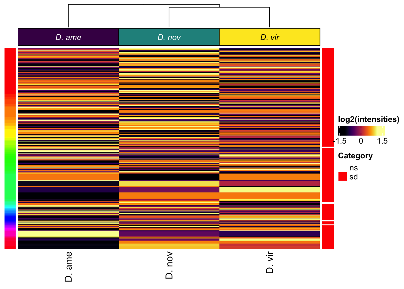
frt_dup_dat %>%
  #filter(Orthogroup %in% da_dup_fem$Orthogroup) %>%
  pivot_longer(cols = 9:11) %>%
  distinct(genes, name, value, .keep_all = TRUE) %>%
  #mutate(species = str_sub(name, 1, 1)) %>%
  ggplot(aes(name, y = value, colour = genes)) +
  geom_line(aes(group = genes), position = position_dodge(width = .25)) +
  geom_jitter(position = position_jitterdodge(dodge.width = .5, jitter.width = .25), alpha = .5) +
  facet_wrap(~ Orthogroup, scales = "free_y") +
  scale_colour_viridis_d() +
  theme_bw() +
  theme(legend.position = '') +
  NULL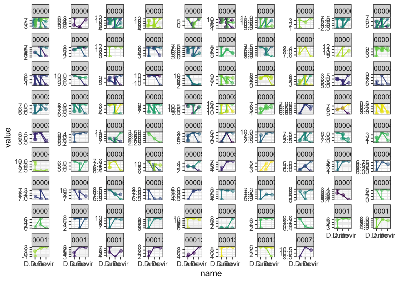
frt_dup_dat %>% filter(Orthogroup %in% da_dup_fem$Orthogroup) %>%
  pivot_longer(cols = 9:11) %>%
  distinct(Orthogroup, genes, name, value) %>%
  group_by(Orthogroup, genes, name) %>%
  summarise(N = n(),
            #mnlfc = mean(logFC),
            mnexp = mean(value),
            sdexp = sd(value)) %>%
  ggplot(aes(name, y = mnexp)) +
  geom_line(aes(group = Orthogroup, colour = Orthogroup)) +
  geom_point(aes(size = N, fill = sdexp), shape = 21) +
  facet_wrap(~ Orthogroup, scales = "free_y") +
  scale_colour_viridis_d(guide = "none") +
  scale_fill_viridis_c() +
  theme_bw() +
  #theme(legend.position = '') +
  NULL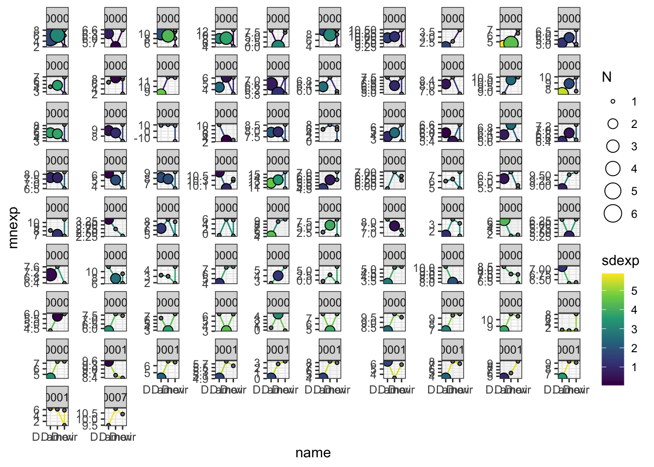
Evolutionary rates
mdb_id <- multiDB %>%
  left_join(vir_fbgn %>% select(-FBtr), by = c('protein_vir' = 'gene_id', "Orthogroup")) %>%
  distinct(protein_vir, .keep_all = TRUE) %>%
  mutate(sigP = if_else(protein_vir %in% vir_sig$protein, "sigP", "not"))

evo_rates <- kaks_results %>%
  filter(Ka.Ks < 10 & !str_detect(COMPARISON, 'lum')) %>%
  distinct(FBgn, COMPARISON, .keep_all = TRUE) %>%
  mutate(signal_cat = case_when(FBgn %in% ejac_cands_multiDB$FBgn[ejac_cands_multiDB$sigP == "sigP"] ~ 'Ejac.signal',
                                FBgn %in% ejac_cands_multiDB$FBgn ~ 'Ejac',
                                FBgn %in% mdb_id$FBgn[mdb_id$sigP == "sigP"] ~ 'FRT.signal',
                                FBgn %in% mdb_id$FBgn ~ 'FRT',
                                TRUE ~ as.character(NA)),
         STEP = if_else(FBgn %in% STEP$FBgn & signal_cat == 'FRT.signal',
                        'STEP', 'other'),
         dupl = if_else(FBgn %in% da_dup$FBgn, "dupl", 'other'))
Signal peptide rates
evo_rates %>%
  drop_na(signal_cat) %>%
  # calculate means and standard errors
  group_by(signal_cat, COMPARISON) %>%
  summarise(N = n(),
            mn = mean(Ka.Ks),
            se = sd(Ka.Ks)/sqrt(N)) %>%

  # add mean for all genes
  bind_rows(
    data.frame(kaks_results %>%
                 dplyr::select(COMPARISON, contains('K')) %>%
                 filter(Ka.Ks < 10 & !str_detect(COMPARISON, 'lum'))) %>%
      group_by(COMPARISON) %>%
      summarise(N = n(),
                mn = mean(Ka.Ks),
                se = sd(Ka.Ks)/sqrt(N)) %>%
      mutate(signal_cat = 'All')
            ) %>%

  mutate(cat2 = str_sub(signal_cat, 1, 3),
         cat3 = if_else(grepl('sig', x = signal_cat) == TRUE, 'Signal pep.', 'Other')) %>%

  # plot
  ggplot(aes(x = factor(cat2, level = c('All', 'FRT', 'Eja')),
             y = mn, colour = COMPARISON, shape = cat3)) +
  geom_point(size = 8, position = position_dodge(width = .8)) +
  geom_errorbar(aes(ymin = mn - se, ymax = mn + se), width = .5, position = position_dodge(width = .8)) +
  scale_colour_manual(values = cbPalette[-1],
                      labels = c(D.amr_vs_D.nov = 'D. ame vs. D. nov',
                                 D.amr_vs_D.vir = 'D. ame vs. D. vir',
                                 D.nov_vs_D.vir = 'D. nov vs. D. vir')) +
  scale_x_discrete(labels = c('All', 'Female reproductive\ntract', 'Ejaculate')) +
  scale_shape_manual(values = c(16, 18)) +
  labs(x = 'category', y = 'dN/dS') +
  theme_bw() +
  theme(text = element_text(size = 20),
        legend.position = c(0.25, 0.75),
        legend.title = element_blank(),
        legend.text = element_text(face = "italic"),
        legend.background = element_rect(fill = NA),
        axis.title.x = element_blank()) +
  #ggsave('plots/TPP_results/all_KaKs.pdf', height = 9, width = 8.5, dpi = 600, useDingbats = FALSE) +
  NULL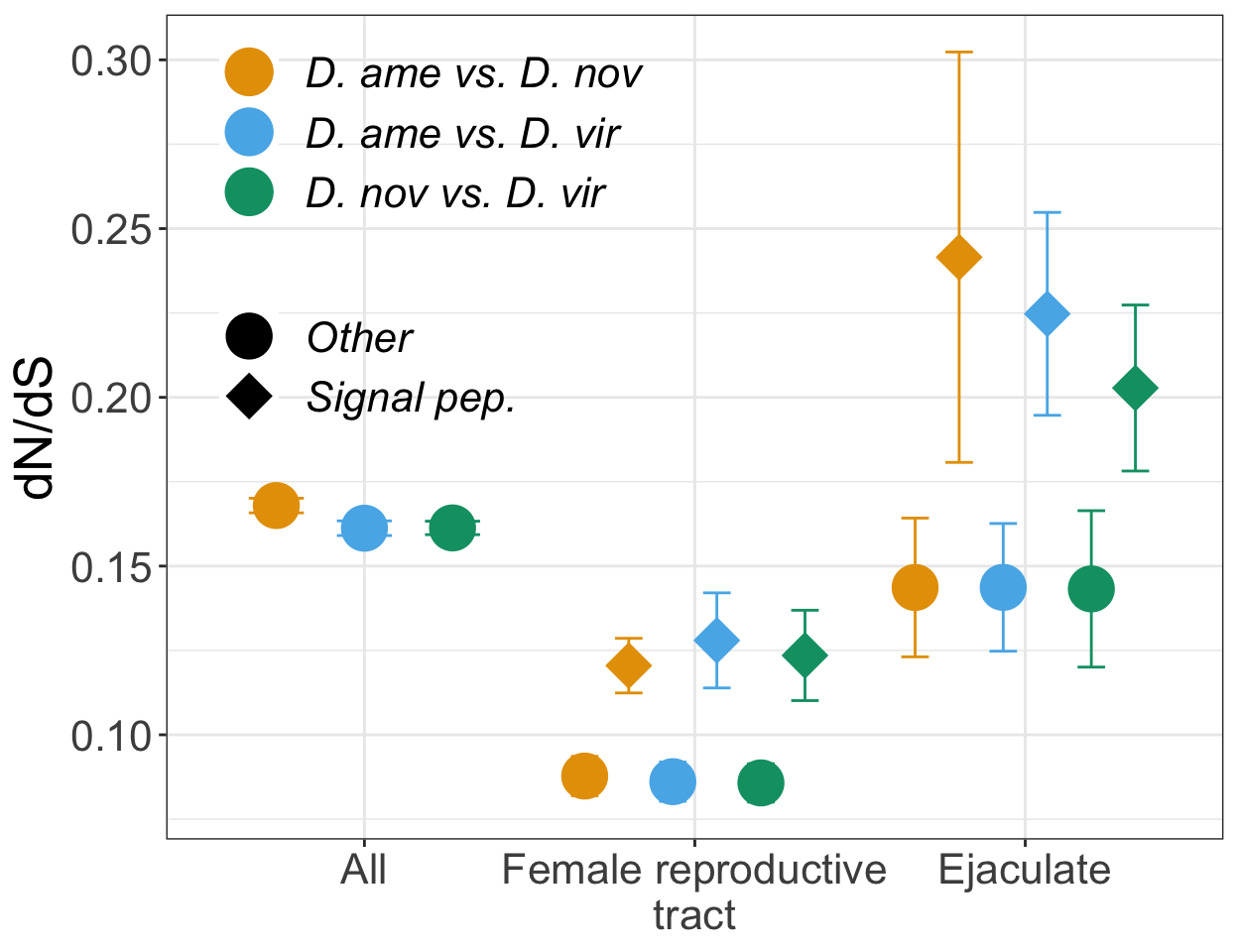
STEP rates
mean_rates <- evo_rates %>%
  group_by(COMPARISON) %>%
  summarise(N = n(),
            mn = mean(Ka.Ks),
            se = sd(Ka.Ks)/sqrt(N)) %>%
  mutate(signal_cat = NA,
         STEP = NA,
         COMPARISON = recode(COMPARISON,
                             D.amr_vs_D.nov = 'D. ame vs. D. nov',
                             D.amr_vs_D.vir = 'D. ame vs. D. vir',
                             D.nov_vs_D.vir = 'D. nov vs. D. vir'))

#plot
evo_rates %>%
  drop_na(signal_cat) %>%
  group_by(signal_cat, STEP, COMPARISON) %>%
  summarise(N = n(),
            mn = mean(Ka.Ks),
            se = sd(Ka.Ks)/sqrt(N)) %>%

  mutate(COMPARISON = recode(COMPARISON,
                             D.amr_vs_D.nov = 'D. ame vs. D. nov',
                             D.amr_vs_D.vir = 'D. ame vs. D. vir',
                             D.nov_vs_D.vir = 'D. nov vs. D. vir')) %>%

  ggplot(aes(x = signal_cat, y = mn, fill = STEP)) +
  geom_hline(data = mean_rates, aes(yintercept = mn), lty = 2, lwd = 1.5) +
  geom_errorbar(aes(ymin = mn - se, ymax = mn + se), position = position_dodge(width = .85),
                width = .5) +
  geom_point(position = position_dodge(width = .85), pch = 21, size = 5) +
  scale_x_discrete(labels = c('Ejac.', 'Ejac.\nsig. pep.',
                              'FRT', 'FRT\nsig. pep.')) +
  scale_fill_manual(values = c('black', 'red')) +
  labs(y = expression(omega)) +
  facet_wrap(~COMPARISON) +
  theme_bw() +
  theme(legend.position = 'bottom',
        legend.title = element_blank(),
        strip.text = element_text(size = 15, face = "italic"),
        axis.title.x = element_blank(),
        axis.title.y = element_text(size = 25),
        axis.text = element_text(size = 15)) +
  geom_text(aes(y = 0.05, label = N), size = 3, position = position_dodge(width = .85)) +
  #ggsave('plots/TPP_results/TPP_STEP_KaKs.pdf', height = 4, width = 9.5, dpi = 600, useDingbats = FALSE) +
  NULL
KW tests
bind_rows(

# Ejac (not signal peptides) vs. genome
evo_rates %>%
  mutate(ejac = if_else(grepl('Ejac$', x = signal_cat), 'ejac', 'other')) %>%
  group_by(COMPARISON) %>%
  # ggplot(aes(x = ejac, y = Ka.Ks)) +
  # stat_summary() + facet_wrap(~COMPARISON)
  do(fit = broom::tidy(wilcox.test(Ka.Ks ~ ejac, data = .))) %>%
  unnest(fit),

# ejac.signal vs. genome
evo_rates %>%
  mutate(ejac = if_else(grepl('Ejac.signal', x = signal_cat), 'ejac', 'other')) %>%
  group_by(COMPARISON) %>%
  # ggplot(aes(x = ejac, y = Ka.Ks)) +
  # stat_summary() + facet_wrap(~COMPARISON)
  do(fit = broom::tidy(wilcox.test(Ka.Ks ~ ejac, data = .))) %>%
  unnest(fit),

# ejac.signal vs. ejac.signal + STEP
evo_rates %>%
  filter(str_detect(signal_cat, 'Ejac.signal')) %>%
  dplyr::select(-STEP) %>%
  mutate(STEP = if_else(FBgn %in% STEP$FBgn, 'STEP', 'other')) %>%
  group_by(COMPARISON) %>%
  # ggplot(aes(x = STEP, y = Ka.Ks)) +
  # stat_summary() + facet_wrap(~COMPARISON)
  do(fit = broom::tidy(wilcox.test(Ka.Ks ~ STEP, data = .))) %>%
  unnest(fit),

# ejac/frt w/o signal peptide
evo_rates %>%
  mutate(sex = case_when(grepl('Ejac', x = signal_cat) ~ 'xEjac',
                         grepl('FRT', x = signal_cat) ~ 'xFRT',
                         TRUE ~ as.character(NA)),
         sigp = if_else(grepl('signal', x = signal_cat), 'sigp', 'other')) %>%
  filter(str_detect(sex, 'x')) %>%
  group_by(sex, COMPARISON) %>%
  # ggplot(aes(x = sex, y = Ka.Ks, colour = sigp)) +
  # stat_summary() + facet_wrap(~COMPARISON)
  do(fit = broom::tidy(wilcox.test(Ka.Ks ~ sigp, data = .))) %>%
  unnest(fit),

# frt (not signal peptides) vs. genome
evo_rates %>%
  mutate(frt = if_else(grepl('FRT$', x = signal_cat), 'frt', 'other')) %>%
  group_by(COMPARISON) %>%
  # ggplot(aes(x = frt, y = Ka.Ks)) +
  # stat_summary() + facet_wrap(~COMPARISON)
  do(fit = broom::tidy(wilcox.test(Ka.Ks ~ frt, data = .))) %>%
  unnest(fit),

# FRT.signal vs. genome
evo_rates %>%
  mutate(frt = if_else(grepl('FRT.signal', x = signal_cat), 'frt', 'other')) %>%
  group_by(COMPARISON) %>%
  # ggplot(aes(x = frt, y = Ka.Ks)) +
  # stat_summary() + facet_wrap(~COMPARISON)
  do(fit = broom::tidy(wilcox.test(Ka.Ks ~ frt, data = .))) %>%
  unnest(fit),

# FRT STEP + signal vs. FRT + signal
evo_rates %>%
  filter(str_detect(signal_cat, 'FRT')) %>%
  # ggplot(aes(x = STEP, y = Ka.Ks)) +
  # stat_summary() + facet_wrap(~COMPARISON)
  group_by(COMPARISON) %>%
  do(fit = broom::tidy(wilcox.test(Ka.Ks ~ STEP, data = .))) %>%
  unnest(fit),

# FRT STEP + signal vs. genome
evo_rates %>%
  mutate(STEP = case_when(STEP == 'STEP' ~ 'frt',
                          TRUE ~ 'other')) %>%
  # ggplot(aes(x = STEP, y = Ka.Ks)) +
  # stat_summary() + facet_wrap(~COMPARISON)
  group_by(COMPARISON) %>%
  do(fit = broom::tidy(wilcox.test(Ka.Ks ~ STEP, data = .))) %>%
  unnest(fit),

# FRT STEP vs. Ejac.signal
evo_rates %>%
  mutate(sex = case_when(grepl('Ejac.signal', x = signal_cat) ~ 'Ejac.sig',
                         STEP == 'STEP' ~ 'STEP',
                         TRUE ~ as.character(NA))) %>%
  drop_na(sex) %>%
  group_by(COMPARISON) %>%
  # ggplot(aes(x = sex, y = Ka.Ks)) +
  # stat_summary() + facet_wrap(~COMPARISON)
  do(fit = broom::tidy(wilcox.test(Ka.Ks ~ sex, data = .))) %>%
  unnest(fit)

) %>%
  mutate(pval = ifelse(p.value < 0.001, '< 0.001', round(p.value, 3)),
         sigLabel = case_when(p.value < 0.001 ~ "***",
                              p.value < 0.01 ~ "**",
                              p.value < 0.05 ~ "\\*",
                              TRUE ~ '')) %>%
  dplyr::select(-c(statistic:sex)) %>%
  kable(caption = 'Mann-Whitney U tests comparing evolutionary rates between groups') %>%
  kable_styling(full_width = FALSE) %>%
  group_rows("Ejaculate (excl. sig. peps.) vs. genome", 1, 3) %>%
  group_rows("Ejaculate sig. peps. vs. genome", 4, 6) %>%
  group_rows("Ejaculate sig. peps. vs. Ejaculate sig. peps. + STEP", 7, 9) %>%
  group_rows("Ejaculate with vs. without sig. peps.", 10, 12) %>%
  group_rows("FRT with vs. without sig. peps.", 13, 15) %>%
  group_rows("FRT (excl. sig. peps.) vs. genome", 16, 18) %>%
  group_rows("FRT sig. peps. vs. genome", 19, 21) %>%
  group_rows("FRT STEP w/ sig. peps. vs. FRT w/ sig. peps.", 22, 24) %>%
  group_rows("FRT STEP w/ sig. peps. vs. genome", 25, 27) %>%
group_rows("FRT STEP vs. Ejac.signal", 28, 30)| COMPARISON | pval | sigLabel |
|---|---|---|
| Ejaculate (excl. sig. peps.) vs. genome | ||
| D.amr_vs_D.nov | 0.218 | |
| D.amr_vs_D.vir | 0.266 | |
| D.nov_vs_D.vir | 0.08 | |
| Ejaculate sig. peps. vs. genome | ||
| D.amr_vs_D.nov | 0.654 | |
| D.amr_vs_D.vir | 0.037 | * |
| D.nov_vs_D.vir | 0.114 | |
| Ejaculate sig. peps. vs. Ejaculate sig. peps. + STEP | ||
| D.amr_vs_D.nov | 0.499 | |
| D.amr_vs_D.vir | 0.06 | |
| D.nov_vs_D.vir | 0.139 | |
| Ejaculate with vs. without sig. peps. | ||
| D.amr_vs_D.nov | 0.202 | |
| D.amr_vs_D.vir | 0.023 | * |
| D.nov_vs_D.vir | 0.012 | * |
| FRT with vs. without sig. peps. | ||
| D.amr_vs_D.nov | < 0.001 | *** |
| D.amr_vs_D.vir | < 0.001 | *** |
| D.nov_vs_D.vir | < 0.001 | *** |
| FRT (excl. sig. peps.) vs. genome | ||
| D.amr_vs_D.nov | < 0.001 | *** |
| D.amr_vs_D.vir | < 0.001 | *** |
| D.nov_vs_D.vir | < 0.001 | *** |
| FRT sig. peps. vs. genome | ||
| D.amr_vs_D.nov | < 0.001 | *** |
| D.amr_vs_D.vir | < 0.001 | *** |
| D.nov_vs_D.vir | < 0.001 | *** |
| FRT STEP w/ sig. peps. vs. FRT w/ sig. peps. | ||
| D.amr_vs_D.nov | 0.008 | ** |
| D.amr_vs_D.vir | 0.001 | ** |
| D.nov_vs_D.vir | 0.003 | ** |
| FRT STEP w/ sig. peps. vs. genome | ||
| D.amr_vs_D.nov | 0.926 | |
| D.amr_vs_D.vir | 0.546 | |
| D.nov_vs_D.vir | 0.86 | |
| FRT STEP vs. Ejac.signal | ||
| D.amr_vs_D.nov | 0.81 | |
| D.amr_vs_D.vir | 0.677 | |
| D.nov_vs_D.vir | 0.558 | |
Database comparisons
Numbers of differentially abundant proteins detected
Here we compare the numbers of differentially abundant proteins detected when using each species databases and the combined database.
Number of ejaculate candidates
Number of proteins more abundant in mated vs. virgin samples
# total number of ejaculate candidates per database
bind_rows(
  ame_DATABLES %>% filter(threshold == 'DA' & str_detect(DA, 'MB')) %>%
    distinct(genes, .keep_all = TRUE),
  nov_DATABLES %>% filter(threshold == 'DA' & str_detect(DA, 'MB')) %>%
    distinct(genes, .keep_all = TRUE),
  vir_DATABLES %>% filter(threshold == 'DA' & str_detect(DA, 'MB')) %>%
    distinct(genes, .keep_all = TRUE),
  comb_TABLES_nd %>% filter(threshold == 'SD' & str_detect(DA, 'MB')) %>%
    distinct(genes, .keep_all = TRUE) %>%
    mutate(threshold = recode(threshold, SD = "DA"), DB = 'aa.comb') %>%
    dplyr::select(species, DB, threshold)) %>%
  group_by(DB) %>%
  dplyr::count() %>%
  left_join(data.frame(DB = c('aa.comb', 'ame.db', 'nov.db', 'vir.db'),
                       total = c(n_distinct(comb_TABLES_nd$genes),
                                 n_distinct(ame_DATABLES$genes),
                                 n_distinct(nov_DATABLES$genes),
                                 n_distinct(vir_DATABLES$genes)))) %>%
  mutate(prop.ejac = n/total)
# A tibble: 4 × 4
# Groups: DB [4]
DB n total prop.ejac
<chr> <int> <int> <dbl>
1 aa.comb 199 2006 0.0992
2 ame.db 257 2838 0.0906
3 nov.db 262 2966 0.0883
4 vir.db 230 2939 0.0783ejac_counts <- bind_rows(
ame_DATABLES %>% filter(threshold == 'DA' & str_detect(DA, 'MB')),
nov_DATABLES %>% filter(threshold == 'DA' & str_detect(DA, 'MB')),
vir_DATABLES %>% filter(threshold == 'DA' & str_detect(DA, 'MB')),
comb_TABLES_nd %>% filter(threshold == 'SD' & str_detect(DA, 'MB')) %>%
mutate(threshold = recode(threshold, SD = "DA"), DB = 'aa.comb') %>%
dplyr::select(species, DB, threshold)) %>%
group_by(species, DB) %>%
dplyr::count()
ejac_counts %>%
ggplot(aes(x = species, y = n, fill = DB)) +
geom_col(position = 'dodge') +
scale_x_discrete(labels = c(expression(italic('D. ame')),
expression(italic('D. nov')),
expression(italic('D. vir')))) +
scale_fill_manual(values = c(viridis::magma(n = 4)[3], viridis::viridis(n = 3)),
name = "Database:",
labels = c('Combined',
expression(italic('D. ame')),
expression(italic('D. nov')),
expression(italic('D. vir')))) +
labs(y = 'No. proteins') +
theme_bw() +
theme(legend.position = 'bottom',
legend.background = element_rect(fill = NA),
axis.title.x = element_blank()) +
#ggsave('plots/database_comps/TPP_comps/TPP_n_ejac_comb.pdf', height = 3, width = 4, dpi = 600, useDingbats = FALSE) +
NULL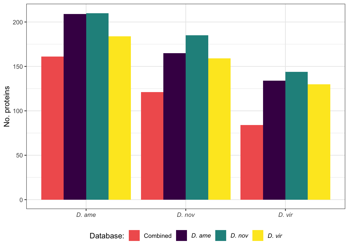
Differentially abundant ejaculate candidates
Number of proteins detected as differentially abundant in pairwise comparisons between species
ejac_da <- bind_rows(ame_MATED %>% filter(threshold == 'DA') %>%
                       dplyr::select(comparison, DB, threshold),
                     nov_MATED %>% filter(threshold == 'DA') %>%
                       dplyr::select(comparison, DB, threshold),
                     vir_MATED %>% filter(threshold == 'DA') %>%
                       dplyr::select(comparison, DB, threshold),
                     mated_TABLES %>% filter(threshold == 'SD') %>%
                       mutate(comparison = recode(comparison,
                                                  aMn = "ame.v.nov",
                                                  aMv = "ame.v.vir",
                                                  nMv = 'nov.v.vir'),
                              threshold = recode(threshold, SD = "DA"),
                              DB = 'aa.comb') %>%
                       dplyr::select(comparison, DB, threshold))

# number of DA ejaculate proteins for each species by database
ejac_da %>%
  group_by(comparison, DB) %>% dplyr::count() %>%
  ggplot(aes(x = comparison, y = n, fill = DB)) +
  geom_col(position = 'dodge') +
  scale_x_discrete(labels = c(expression(italic('D. ame vs. D. nov')),
                              expression(italic('D. ame vs. D. vir')),
                              expression(italic('D. nov vs. D. vir')))) +
  scale_fill_manual(values = c(viridis::magma(n = 4)[3], viridis::viridis(n = 3)),
                    name = "Database:",
                    labels = c('Combined',
                               expression(italic('D. ame')),
                               expression(italic('D. nov')),
                               expression(italic('D. vir')))) +
  labs(y = 'No. proteins') +
  theme_bw() +
  theme(legend.position = 'bottom',
        legend.background = element_rect(fill = NA),
        axis.title.x = element_blank()) +
  #ggsave('plots/database_comps/TPP_comps/TPP_n_DA_comb.pdf', height = 3, width = 4, dpi = 600, useDingbats = FALSE) +
  NULL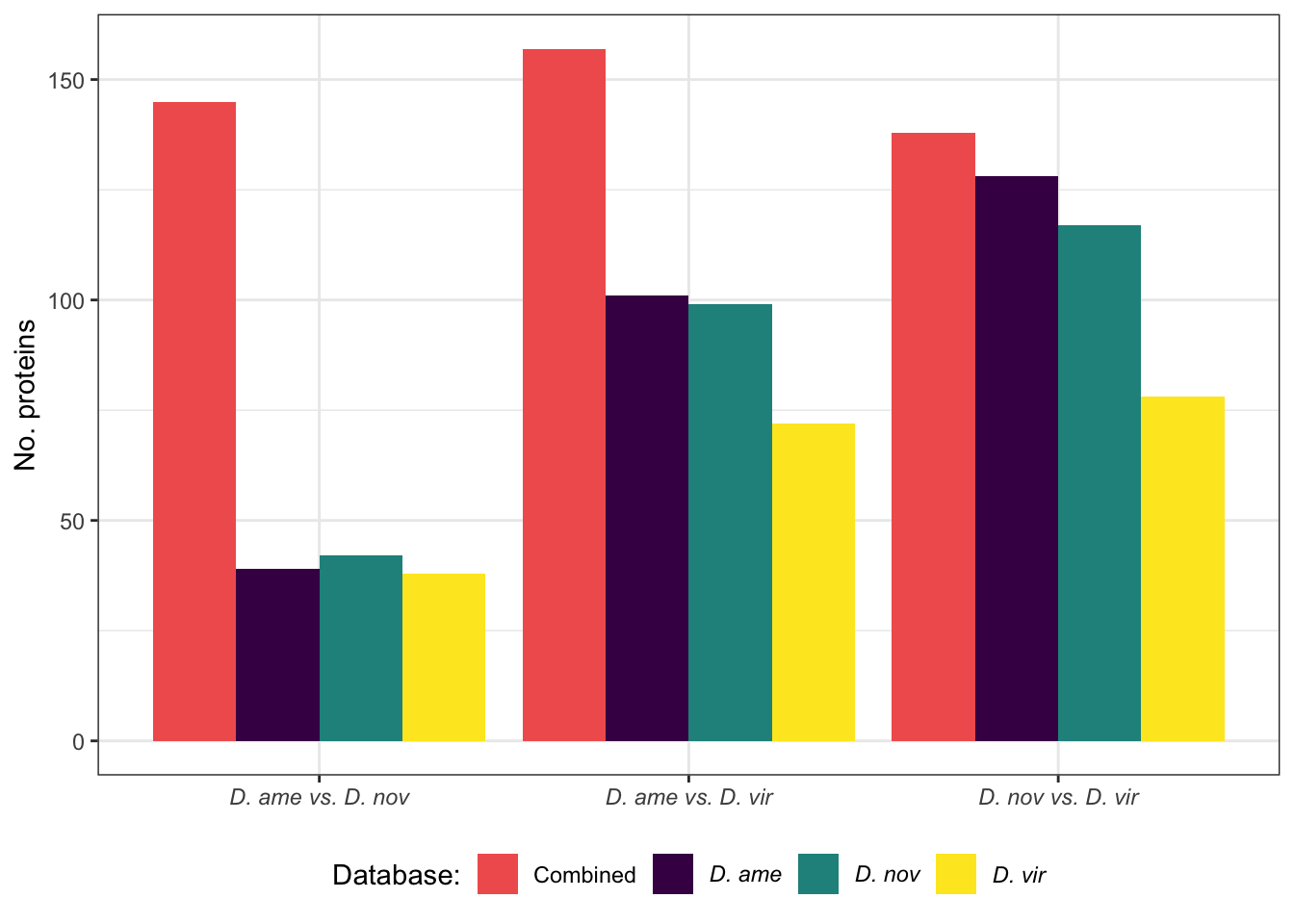
Differentially abundant female reproductive tract proteins
Number of proteins detected as differentially abundant in pairwise comparisons between species
frt_da <- bind_rows(ame_VIRGIN %>% filter(threshold == 'DA') %>%
                      dplyr::select(comparison, DB, threshold),
                    nov_VIRGIN %>% filter(threshold == 'DA') %>%
                      dplyr::select(comparison, DB, threshold),
                    vir_VIRGIN %>% filter(threshold == 'DA') %>%
                      dplyr::select(comparison, DB, threshold),
                    fem_TABLES %>% filter(threshold == 'SD') %>%
                      mutate(comparison = recode(comparison,
                                                 aVn = "ame.v.nov",
                                                 aVv = "ame.v.vir",
                                                 nVv = 'nov.v.vir'),
                             threshold = recode(threshold, SD = "DA"),
                             DB = 'aa.comb') %>%
                      dplyr::select(comparison, DB, threshold))

frt_da %>%
  group_by(comparison, DB) %>% dplyr::count() %>%
  ggplot(aes(x = comparison, y = n, fill = DB)) +
  geom_col(position = 'dodge') +
  scale_x_discrete(labels = c(expression(italic('D. ame vs. D. nov')),
                              expression(italic('D. ame vs. D. vir')),
                              expression(italic('D. nov vs. D. vir')))) +
  scale_fill_manual(values = c(viridis::magma(n = 4)[3], viridis::viridis(n = 3)),
                    name = "Database:",
                    labels = c('Combined',
                               expression(italic('D. ame')),
                               expression(italic('D. nov')),
                               expression(italic('D. vir')))) +
  labs(y = 'No. proteins') +
  theme_bw() +
  theme(legend.position = 'bottom',
        legend.background = element_rect(fill = NA),
        axis.title.x = element_blank()) +
  #ggsave('plots/database_comps/TPP_comps/TPP_n_DAfem_comb.pdf', height = 3, width = 4, dpi = 600, useDingbats = FALSE) +
  NULL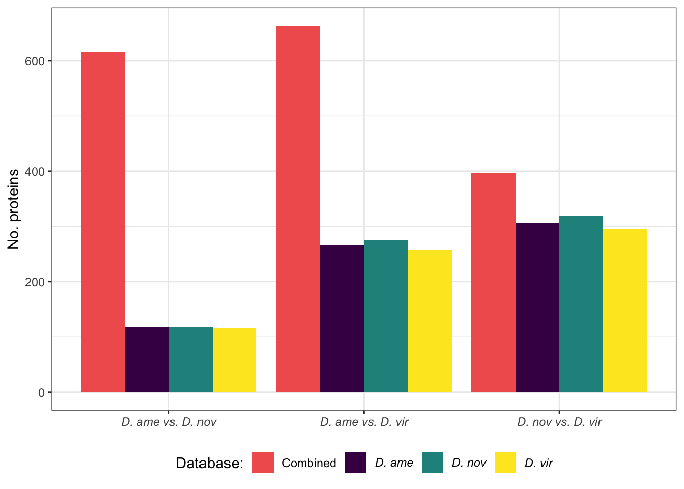
Proportions detected
bind_rows(ejac_counts %>%
            left_join(data.frame(DB = c('aa.comb', 'ame.db', 'nov.db', 'vir.db'),
                                 total = c(n_distinct(comb_TABLES_nd$genes),
                                           n_distinct(ame_DATABLES$genes),
                                           n_distinct(nov_DATABLES$genes),
                                           n_distinct(vir_DATABLES$genes)))) %>%
            mutate(set = 'Ejaculate candidates',
                   comparison = species),
          ejac_da %>%
            group_by(comparison, DB) %>% dplyr::count() %>%
            left_join(data.frame(DB = c('aa.comb', 'ame.db', 'nov.db', 'vir.db'),
                                 total = c(n_distinct(mated_TABLES$genes),
                                           n_distinct(ame_MATED$genes),
                                           n_distinct(nov_MATED$genes),
                                           n_distinct(vir_MATED$genes)))) %>%
            mutate(set = 'Ejaculate divergence'),
          frt_da %>%
            group_by(comparison, DB) %>% dplyr::count() %>%
            left_join(data.frame(DB = c('aa.comb', 'ame.db', 'nov.db', 'vir.db'),
                                 total = c(n_distinct(fem_TABLES$genes),
                                           n_distinct(ame_VIRGIN$genes),
                                           n_distinct(nov_VIRGIN$genes),
                                           n_distinct(vir_VIRGIN$genes)))) %>%
            mutate(set = 'FRT divergence')) %>%
  mutate(prop.da = n/total) %>%
  ggplot(aes(x = comparison, y = prop.da, colour = DB)) +
  geom_line(aes(group = DB), lwd = 2) +
  scale_x_discrete(labels = c(expression(italic('D. ame vs. D. nov')),
                              expression(italic('D. ame vs. D. vir')),
                              expression(italic('D. nov vs. D. vir')))) +
  scale_y_continuous(labels = scales::percent) +
  scale_colour_manual(values = c(viridis::magma(n = 4)[3], viridis::viridis(n = 3)),
                      name = "Database",
                      labels = c('Combined',
                                 expression(italic('D. ame')),
                                 expression(italic('D. nov')),
                                 expression(italic('D. vir')))) +
  labs(y = '% differentially abundant') +
  facet_wrap(~set, scales = 'free', nrow = 1) +
  theme_bw() +
  theme(#legend.position = 'bottom',
        legend.text.align = 0,
        legend.background = element_rect(fill = NA),
        axis.title.x = element_blank(),
        axis.text.x = element_text(size = 8),
        strip.text = element_text(size = 15)) +
  #ggsave('plots/database_comps/TPP_comps/TPP_prop_DA.pdf', height = 3.8, width = 13.5, dpi = 600, useDingbats = FALSE) +
  NULL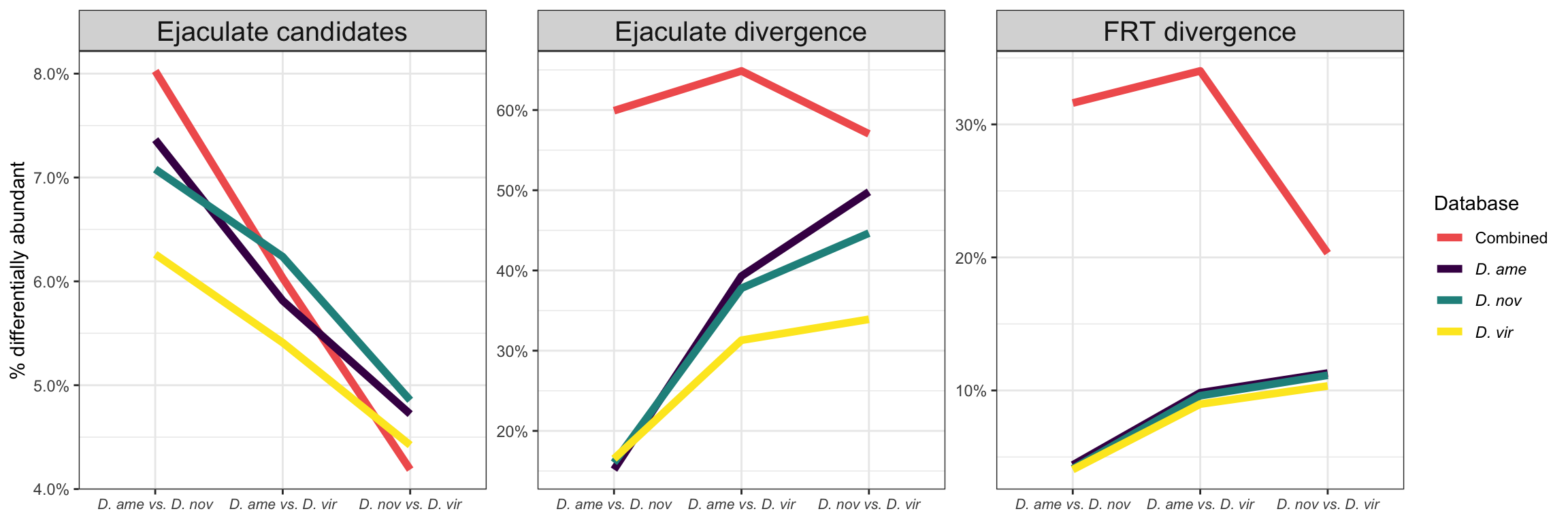
Abundance correlations
Here we compare the protein abundances when searching against each
species proteome. First, we average the abundances for each search by
taking the mean across all three replicates of AM
(1-3).
all_abund <- mdb2 %>%
  select(protein_vir, #FBgn,
         starts_with('AV'), starts_with('AM'),
         starts_with('NV'), starts_with('NM'),
         starts_with('VV'), starts_with('VM'))

abund_cor <- bind_rows(
  # correlations between replicates within treatment using species specific DB
  all_abund %>% dplyr::select(-protein_vir) %>% +1 %>% log2 %>% cor(use = "complete.obs") %>%
  reshape2::melt() %>%
  mutate(condition1 = str_sub(Var1, 1, 2),
         condition2 = str_sub(Var2, 1, 2),
         sample1 = str_sub(Var1, 1, 3),
         sample2 = str_sub(Var2, 1, 3),
         db1 = str_sub(Var1, 5, 7),
         db2 = str_sub(Var2, 5, 7)) %>%
  filter(condition1 == condition2) %>%
  filter(Var1 != Var2) %>%
  filter(db1 == db2) %>%
  distinct(value, .keep_all = TRUE) %>%

  # calculate means and standard errors
  group_by(condition1, db1, db2) %>%
  summarise(N = n(),
            mn = mean(value),
            se = sd(value)/sqrt(N)) %>%
  filter(str_sub(tolower(condition1), 1, 1) == str_sub(db1, 1, 1)),

  # correlations between replicates using alt. species DB
  all_abund %>% dplyr::select(-protein_vir) %>% +1 %>% log2 %>% cor(use = "complete.obs") %>%
  reshape2::melt() %>%
  mutate(condition1 = str_sub(Var1, 1, 2),
         condition2 = str_sub(Var2, 1, 2),
         sample1 = str_sub(Var1, 1, 3),
         sample2 = str_sub(Var2, 1, 3),
         db1 = str_sub(Var1, 5, 7),
         db2 = str_sub(Var2, 5, 7)) %>%
  filter(sample1 == sample2) %>%
  filter(db1 != db2) %>%
  distinct(Var1, Var2, .keep_all = TRUE) %>%

  # calculate means and standard errors
  group_by(condition1, db1, db2) %>%
  summarise(N = n(),
            mn = mean(value),
            se = sd(value)/sqrt(N)) %>%
  filter(str_sub(tolower(condition1), 1, 1) == str_sub(db1, 1, 1))
  )

abund_cor$NAMEX <- c('AMA', 'AVA', 'NMN', 'NVN', 'VMV', 'VVV',
                     'AMN', 'AMV', 'AVN', 'AVV', 'NMA', 'NMV',
                     'NVA', 'NVV', 'VMA', 'VMN', 'VVA', 'VVN')

# plot
abund_cor %>%
  ggplot(aes(x = condition1, y = mn, colour = db2)) +
  geom_errorbar(aes(ymin = mn - se, ymax = mn + se), width = .5) +
  geom_point(size = 5)  +
  labs(y = 'Pearson\'s correlation') +
  scale_colour_viridis_d(name = "Database:",
                         labels = c(expression(italic('D. ame')),
                                    expression(italic('D. nov')),
                                    expression(italic('D. vir')))) +
  theme_bw() +
  theme(legend.position = 'bottom',
        legend.text.align = 0,
        axis.title.x = element_blank()) +
  #ggsave('plots/database_comps/TPP_comps/TPP_abun_correlations.pdf', height = 4.25, width = 4, dpi = 600, useDingbats = FALSE) +
  NULL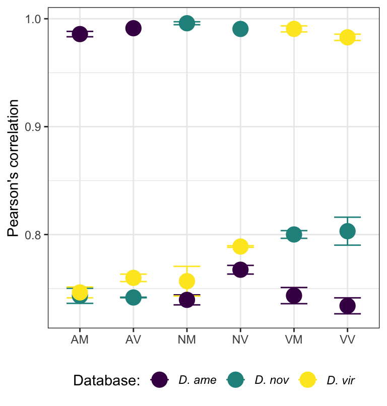
Coefficients of variation
We calculate the coefficient of variation for each treatment (mated or virgin within each species); (1) between biological replicates within each treatment using each species database as a measure of precision and (2) between each sample using each database as a measure of variation between databases.
# function to calculate CV
cv <- function(x) sd(x, na.rm = TRUE)/mean(x, na.rm = TRUE)

# combine data across individual databases
all_vals <- bind_rows(tmt_ame_prot %>%
                        dplyr::select(protein, AM1:VV3) %>%
                        rename_with(.cols = 2:17, function(x) {paste0('ame.', x)}) %>%
                        pivot_longer(2:17),
                      tmt_nov_prot %>%
                        dplyr::select(protein, AM1:VV3) %>%
                        rename_with(.cols = 2:17, function(x) {paste0('nov.', x)}) %>%
                        pivot_longer(2:17),
                      tmt_vir_prot %>%
                        dplyr::select(protein, AM1:VV3) %>%
                        rename_with(.cols = 2:17, function(x) {paste0('vir.', x)}) %>%
                        pivot_longer(2:17)) %>%
  mutate(log_val = log10(value + 1),
         db = str_sub(name, 1, 3),
         condition = str_sub(name, 5, 6),
         .sample = str_sub(name, 5, 7))

# CV for entire experiment using each database
all_vals %>%
  group_by(protein, db) %>%
  summarise(CV = cv(log_val)) %>%
  group_by(db) %>%
  summarise(N = n(),
            md = median(CV, na.rm = TRUE),
            mn = mean(CV, na.rm = TRUE),
            se = sd(CV, na.rm = TRUE)/sqrt(N)) %>%
  ggplot(aes(x = db, y = mn, fill = db)) +
  geom_errorbar(aes(ymin = mn - se, ymax = mn + se), width = 0) +
  geom_point(pch = 21, size = 5) +
  scale_fill_viridis_d() +
  scale_x_discrete(labels = c('ame' = expression(italic('D. ame')),
                              'nov' = expression(italic('D. nov')),
                              'vir' = expression(italic('D. vir')))) +
  labs(x = 'Database', y = 'CV') +
  theme_bw() +
  theme(legend.position = '') +
  NULL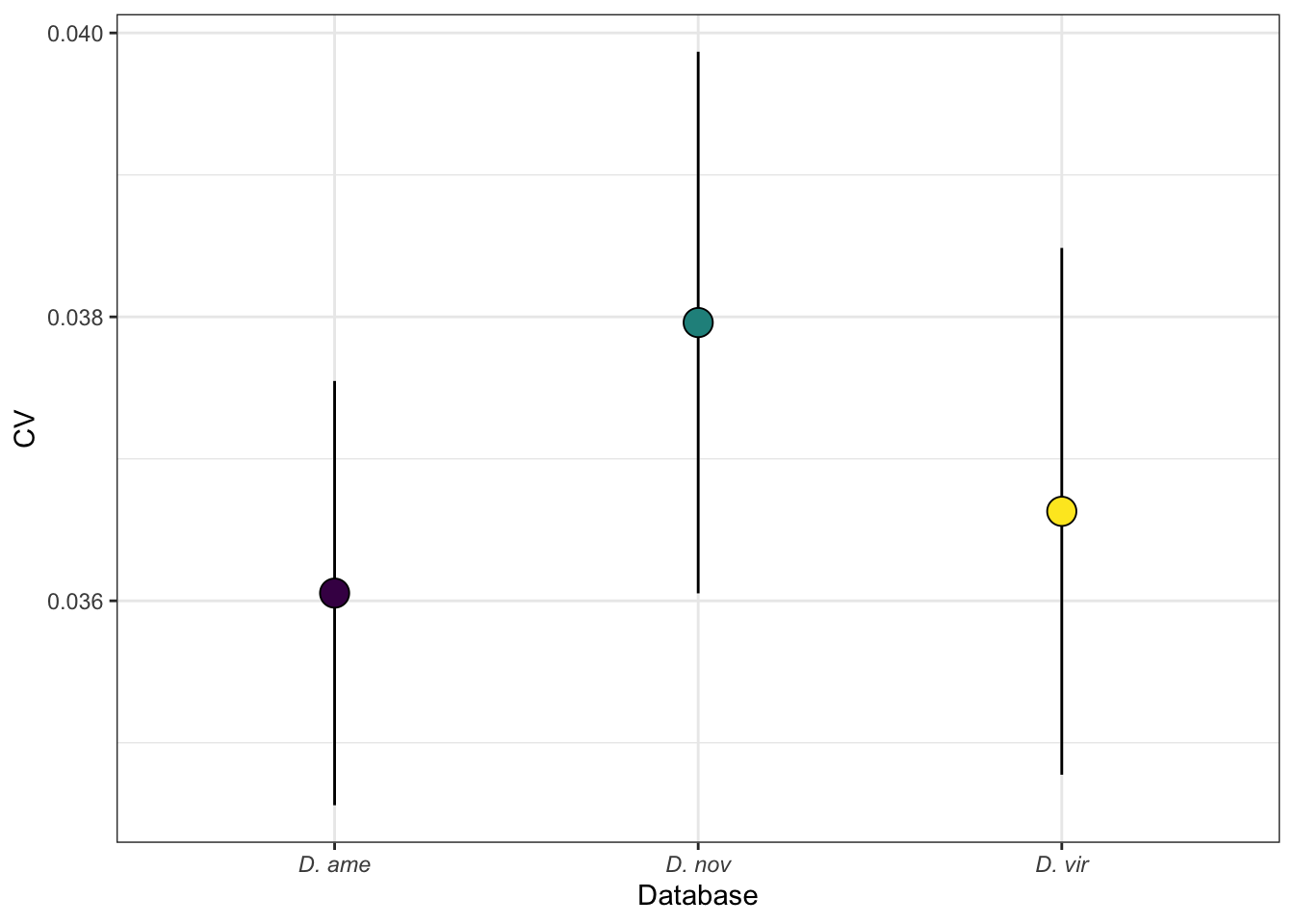
# compare CVs within each condition using each database
all_vals %>%
  group_by(protein, db, condition) %>%
  summarise(CV = cv(log_val)) %>%
  group_by(db, condition) %>%
  summarise(N = n(),
            md = median(CV, na.rm = TRUE),
            mn = mean(CV, na.rm = TRUE),
            se = sd(CV, na.rm = TRUE)/sqrt(N)) %>%
  ggplot(aes(x = condition, y = mn, fill = db)) +
  geom_errorbar(aes(ymin = mn - se, ymax = mn + se), width = 0,
                position = position_dodge(width = .5)) +
  geom_point(pch = 21, position = position_dodge(width = .5)) +
  scale_fill_viridis_d(name = "Database:",
                       labels = c('ame' = expression(italic('D. ame')),
                                  'nov' = expression(italic('D. nov')),
                                  'vir' = expression(italic('D. vir')))) +
  labs(y = 'CV') +
  theme_bw() +
  theme(legend.position = 'bottom') +
  #ggsave('plots/database_comps/TPP_comps/TPP_CV_within_treatment_db.pdf', height = 8, width = 12, units = 'cm', dpi = 600, useDingbats = FALSE) +
  NULL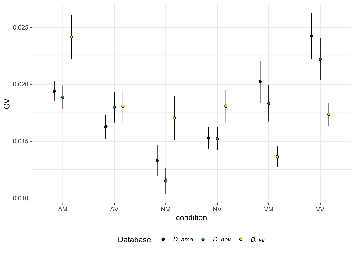
# compare samples across different databases using the combined database to allow comparison between the same proteins across databases.
all_abund %>%
  pivot_longer(2:49) %>%
  mutate(log_val = log10(value),
         db = str_sub(name, 5, 7),
         condition = str_sub(name, 1, 2),
         .sample = str_sub(name, 1, 3)) %>%
  group_by(protein_vir, .sample) %>%
  summarise(CV = cv(log_val)) %>%
  group_by(.sample) %>%
  summarise(N = n(),
            md = median(CV, na.rm = TRUE),
            mn = mean(CV, na.rm = TRUE),
            se = sd(CV, na.rm = TRUE)/sqrt(N)) %>%
  ggplot(aes(x = .sample, y = mn)) +
  geom_errorbar(aes(ymin = mn - se, ymax = mn + se), width = 0) +
  geom_point(size = 5) +
  labs(y = 'CV') +
  theme_bw() +
  theme(legend.position = 'bottom') +
  #ggsave('plots/database_comps/TPP_comps/TPP_CV_btw_sample_db.pdf', height = 5, width = 15, units = 'cm', dpi = 600, useDingbats = FALSE) +
  NULL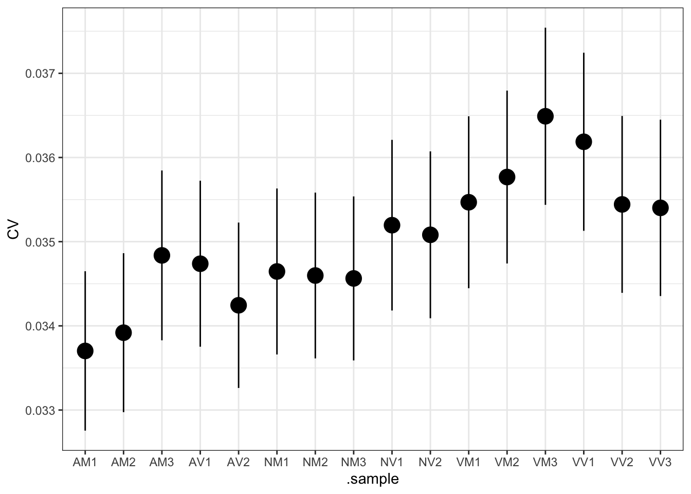
Test differences in abundances between databases
We compared differences in abundance between databases for each species/mating combination using edgeR. Significant differences in abundance indicate that using each species data provides different estimates of protein abundance.
Heatmap
abun_mn <- all_abund %>%
  mutate(mn = rowMeans(dplyr::select(., -c(1)), na.rm = TRUE)) %>%
  filter(mn > 0) %>%
  mutate(AMA = rowMeans(dplyr::select(., matches("AM._ame")), na.rm = TRUE),
         AVA = rowMeans(dplyr::select(., matches("AV._ame")), na.rm = TRUE),
         AMN = rowMeans(dplyr::select(., matches("AM._nov")), na.rm = TRUE),
         AVN = rowMeans(dplyr::select(., matches("AV._nov")), na.rm = TRUE),
         AMV = rowMeans(dplyr::select(., matches("AM._vir")), na.rm = TRUE),
         AVV = rowMeans(dplyr::select(., matches("AV._vir")), na.rm = TRUE),

         NMA = rowMeans(dplyr::select(., matches("NM._ame")), na.rm = TRUE),
         NVA = rowMeans(dplyr::select(., matches("NV._ame")), na.rm = TRUE),
         NMN = rowMeans(dplyr::select(., matches("NM._nov")), na.rm = TRUE),
         NVN = rowMeans(dplyr::select(., matches("NV._nov")), na.rm = TRUE),
         NMV = rowMeans(dplyr::select(., matches("NM._vir")), na.rm = TRUE),
         NVV = rowMeans(dplyr::select(., matches("NV._vir")), na.rm = TRUE),

         VMA = rowMeans(dplyr::select(., matches("VM._ame")), na.rm = TRUE),
         VVA = rowMeans(dplyr::select(., matches("VV._ame")), na.rm = TRUE),
         VMN = rowMeans(dplyr::select(., matches("VM._nov")), na.rm = TRUE),
         VVN = rowMeans(dplyr::select(., matches("VV._nov")), na.rm = TRUE),
         VMV = rowMeans(dplyr::select(., matches("VM._vir")), na.rm = TRUE),
         VVV = rowMeans(dplyr::select(., matches("VV._vir")), na.rm = TRUE)) %>%
  dplyr::select(protein_vir, AMA:VVV) %>%
  drop_na(AMA:VVV)

# scale data
scaled_comp <- as.matrix(pheatmap:::scale_rows(log2(abun_mn[, -1] + 1)))

colnames(scaled_comp) <- colnames(abun_mn[, -1])

sp_anno <- str_sub(colnames(abun_mn[, -1]), 1, 1)
mt_anno <- str_sub(colnames(abun_mn[, -1]), 2, 2)
db_anno <- str_sub(colnames(abun_mn[, -1]), 3, 3)

# get column names for ordering
v <- colnames(scaled_comp)

ha <- HeatmapAnnotation(
  species = str_sub(colnames(abun_mn[, -1]), 1, 1),
  mating = str_sub(colnames(abun_mn[, -1]), 2, 2),
  database = str_sub(colnames(abun_mn[, -1]), 3, 3),
  col = list(species = c('V' = v.pal[1],
                         'N' = v.pal[2],
                         'A' = v.pal[3]),
             mating = c('M' = viridis::magma(n = 4)[3],
                        'V' = viridis::magma(n = 4)[2]),
             database = c('V' = v.pal[1],
                          'N' = v.pal[2],
                          'A' = v.pal[3])
             )
  # cors = anno_points(
  #   abund_cor[match(v[order(substr(v, start = 1,
  #                                  stop = max(nchar(v))))], abund_cor$NAMEX), 'mn'])
  )

#pdf('plots/database_comps/TPP_comps/TPP_db_comp_compheatmap.pdf', height = 8, width = 5)
Heatmap(scaled_comp,
        col = RColorBrewer::brewer.pal(name = 'Spectral', n = 10),
        heatmap_legend_param = list(title = "log2(intensities)",
                                    title_position = "leftcenter-rot"),
        column_order = v[order(substr(v, start = 1, stop = max(nchar(v))))],
        #right_annotation = frt_labs,
        #left_annotation = frt_lab,
        top_annotation = ha,
        show_row_names = FALSE,
        show_column_names = FALSE,
        column_gap = unit(0, "mm"),
        row_title = NULL,
        column_title = NULL)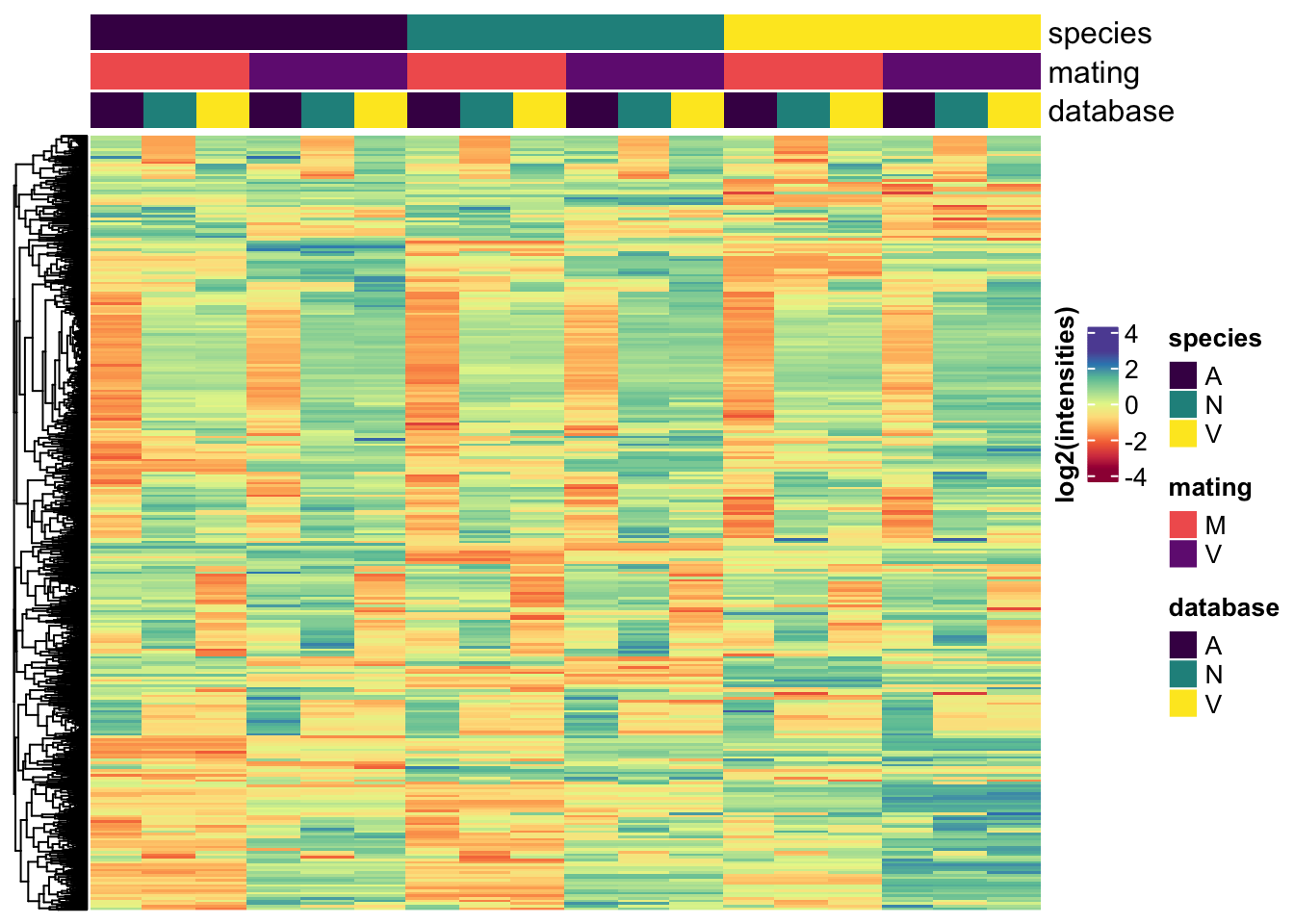
#dev.off()Differential abundance analysis
# subset data for each condition using all databases
am_dat <- all_abund %>% dplyr::select(protein_vir, starts_with('AM')) %>%
  mutate(across(2:10, ~replace_na(.x, 0)))
av_dat <- all_abund %>% dplyr::select(protein_vir, starts_with('AV')) %>%
  mutate(across(2:7, ~replace_na(.x, 0)))

nm_dat <- all_abund %>% dplyr::select(protein_vir, starts_with('NM')) %>%
  mutate(across(2:10, ~replace_na(.x, 0)))
nv_dat <- all_abund %>% dplyr::select(protein_vir, starts_with('NV')) %>%
  mutate(across(2:7, ~replace_na(.x, 0)))

vm_dat <- all_abund %>% dplyr::select(protein_vir, starts_with('VM')) %>%
  mutate(across(2:10, ~replace_na(.x, 0)))
vv_dat <- all_abund %>% dplyr::select(protein_vir, starts_with('VV')) %>%
  mutate(across(2:10, ~replace_na(.x, 0)))

# function to perform differential abundance analysis between databases for the
# same samples

do_limma <- function(df) {

  expr_dat = df[, -1]

  # get sample info
  sampInfo = data.frame(database = str_sub(colnames(expr_dat), 5, 7),
                        Replicate = str_sub(colnames(expr_dat), 3, 3))

  # make design matrix to test diffs between groups
  design = model.matrix(~0 + sampInfo$database)
  colnames(design) = unique(sampInfo$database)
  rownames(design) = sampInfo$Replicate

  # create DGElist and fit model
  dgeList = DGEList(counts = expr_dat, genes = df$protein_vir, group = sampInfo$database)
  dgeList = calcNormFactors(dgeList, method = 'TMM')
  dgeList = estimateCommonDisp(dgeList)
  dgeList = estimateTagwiseDisp(dgeList)

  # make contrasts - higher values = higher alphabetically
  cont.matrix = makeContrasts(a.vs.n = ame - nov,
                              a.vs.v = ame - vir,
                              n.vs.v = nov - vir,
                              levels = design)

  # voom normalisation
  dgeListV = voom(dgeList, design, plot = FALSE)

  # fit linear model
  lm_fit <- lmFit(dgeListV, design = design)

  # compare differential abundance between databases
  # ame vs. nov
  lm_an = contrasts.fit(lm_fit, cont.matrix[,"a.vs.n"])
  lm_an = eBayes(lm_an)
  lm_an.tTags.table = topTable(lm_an, adjust.method = "BH", number = Inf) %>%
    mutate(comparison = "a.vs.n",
           threshold = if_else(adj.P.Val < 0.05 & abs(logFC) > 1, "SD", "NS"))

  # ame vs. vir
  lm_av <- contrasts.fit(lm_fit, cont.matrix[,"a.vs.v"])
  lm_av <- eBayes(lm_av)
  lm_av.tTags.table <- topTable(lm_av, adjust.method = "BH", number = Inf) %>%
    mutate(comparison = "a.vs.v",
           threshold = if_else(adj.P.Val < 0.05 & abs(logFC) > 1, "SD", "NS"))

  # nov vs. vir
  lm_nv <- contrasts.fit(lm_fit, cont.matrix[,"n.vs.v"])
  lm_nv <- eBayes(lm_nv)
  lm_nv.tTags.table <- topTable(lm_nv, adjust.method = "BH", number = Inf) %>%
    mutate(comparison = "n.vs.v",
           threshold = if_else(adj.P.Val < 0.05 & abs(logFC) > 1, "SD", "NS"))

  # combine results
  return(rbind(lm_an.tTags.table, lm_av.tTags.table, lm_nv.tTags.table))

}

# do tests
combi_2 <- bind_rows(do_limma(am_dat) %>% mutate(dat = 'AM'),
                     do_limma(av_dat) %>% mutate(dat = 'AV'),
                     do_limma(nm_dat) %>% mutate(dat = 'NM'),
                     do_limma(nv_dat) %>% mutate(dat = 'NV'),
                     do_limma(vm_dat) %>% mutate(dat = 'VM'),
                     do_limma(vv_dat) %>% mutate(dat = 'VV')) %>%
  left_join(vir_fbgn, by = c('genes' = 'gene_id')) %>%
  mutate(comparison = recode(comparison,
                             a.vs.n = "D.amr_vs_D.nov",
                             a.vs.v = "D.amr_vs_D.vir",
                             n.vs.v = 'D.nov_vs_D.vir')) %>%
  # add evolutionary rates
  left_join(kaks_results %>% dplyr::select(Ka:COMPARISON, FBgn),
            by = c('FBgn', c('comparison' = 'COMPARISON'))) %>%
  distinct(FBgn, comparison, dat, .keep_all = TRUE)

# volcanos
combi_2 %>%
  ggplot(aes(x = logFC, y = -log10(P.Value), colour = threshold)) +
  geom_point(alpha = .5) +
  labs(y = '-log10(p-value)') +
  facet_grid(dat~comparison) +
  theme_bw() +
  theme(legend.position = '') +
  NULL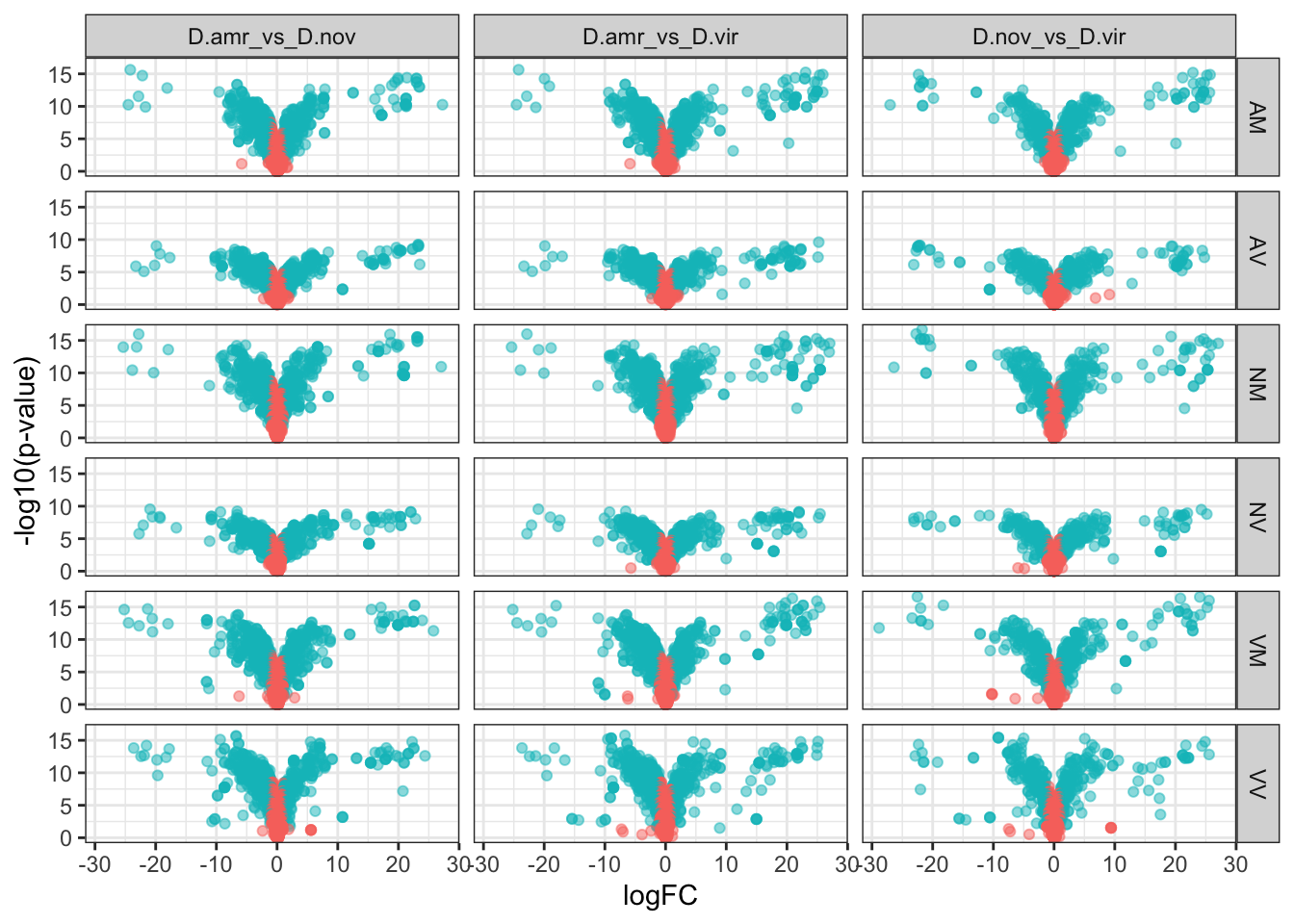
# # numbers differentially abundant
# combi_2 %>%
#   group_by(dat, comparison) %>%
#   count(threshold) %>%
#   ggplot(aes(x = comparison, y = n, fill = threshold)) +
#   geom_col() +
#   facet_wrap(~dat)
#
# # percent different in estimate
# combi_2 %>%
#   group_by(dat, comparison) %>%
#   count(threshold) %>%
#   group_by(dat, comparison) %>%
#   summarise(p.diff = 100 * n[threshold == 'SD']/(n[threshold == 'SD'] + n[threshold == 'NS'])) %>%
#   summary
Evolutionary rates
We compare dN/dS for proteins that showed differences in abundance when using each species database. We expect faster evolving proteins will be more likely differentially abundant between databases if amino acid substitutions lead to less accurate peptide assignment/abundance estimates.
combi_2 %>% filter(Ka.Ks < 10) %>%
  mutate(condition = str_sub(dat, 2, 2)) %>%
  group_by(comparison, threshold, condition) %>%
  summarise(N = n(),
            mn = mean(Ka.Ks),
            se = sd(Ka.Ks)/sqrt(N)) %>%
  ggplot(aes(x = comparison, y = mn, fill = threshold, shape = condition)) +
  geom_errorbar(aes(ymin = mn - se, ymax = mn + se), width = 0,
                position = position_dodge(width = .5)) +
  geom_point(size = 3, position = position_dodge(width = .5)) +
  labs(x = 'Database comparison', y = expression(omega)) +
  scale_shape_manual(values = c(21:22),
                     labels = c('M' = 'Mated',
                                'V' = 'Virgin')) +
  scale_fill_manual(values = cbPalette[-1]) +
  scale_x_discrete(labels =
                     c('D.amr_vs_D.nov' =
                         expression(paste(italic('D. ame'), ' vs. ', italic('D. nov'))),
                       'D.amr_vs_D.vir' =
                         expression(paste(italic('D. ame'), ' vs. ', italic('D. vir'))),
                       'D.nov_vs_D.vir' =
                         expression(paste(italic('D. nov'), ' vs. ', italic('D. vir'))))) +
  guides(fill = guide_legend(override.aes = list(shape = 21))) +
  theme_bw() +
  theme(#legend.position = 'bottom',
        legend.title = element_blank(),
        axis.text.x = element_text(angle = 15, hjust = 1),
        axis.title.y = element_text(size = 25)) +
  #ggsave('plots/database_comps/TPP_comps/TPP_db_comp_rates.pdf', height = 9, width = 11, units = 'cm', dpi = 600, useDingbats = FALSE) +
  NULL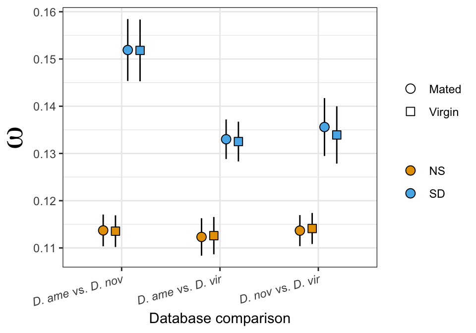
# perform KW tests
kw_rates <- combi_2 %>% filter(Ka.Ks < 10) %>%
  group_by(dat, comparison) %>%
  do(fit = broom::tidy(wilcox.test(Ka.Ks ~ threshold, data = .))) %>%
  unnest(fit)

kw_rates$FDR <- p.adjust(kw_rates$p.value, method = 'fdr')

kw_rates %>%
  mutate(FDR = ifelse(FDR < 0.001, '< 0.001', round(FDR, 3)),
         sigLabel = case_when(FDR < 0.001 ~ "***",
                              FDR < 0.01 ~ "**",
                              FDR < 0.05 ~ "\\*",
                              TRUE ~ '')) %>%
  dplyr::select(-c(p.value:alternative)) %>%
  kable(digits = 3,
        caption = 'Wilcoxon rank sum test with continuity correction') %>%
kable_styling(full_width = FALSE)| dat | comparison | statistic | FDR | sigLabel |
|---|---|---|---|---|
| AM | D.amr_vs_D.nov | 734584.5 | < 0.001 | *** |
| AM | D.amr_vs_D.vir | 767478.0 | < 0.001 | *** |
| AM | D.nov_vs_D.vir | 530712.0 | 0.017 | * |
| AV | D.amr_vs_D.nov | 751014.5 | < 0.001 | *** |
| AV | D.amr_vs_D.vir | 762942.0 | < 0.001 | *** |
| AV | D.nov_vs_D.vir | 514985.5 | 0.005 | ** |
| NM | D.amr_vs_D.nov | 745570.5 | < 0.001 | *** |
| NM | D.amr_vs_D.vir | 752606.5 | < 0.001 | *** |
| NM | D.nov_vs_D.vir | 514221.0 | 0.004 | ** |
| NV | D.amr_vs_D.nov | 748220.5 | < 0.001 | *** |
| NV | D.amr_vs_D.vir | 756255.0 | < 0.001 | *** |
| NV | D.nov_vs_D.vir | 517407.0 | 0.007 | ** |
| VM | D.amr_vs_D.nov | 739669.0 | < 0.001 | *** |
| VM | D.amr_vs_D.vir | 768722.5 | < 0.001 | *** |
| VM | D.nov_vs_D.vir | 518474.0 | 0.019 | * |
| VV | D.amr_vs_D.nov | 751389.5 | < 0.001 | *** |
| VV | D.amr_vs_D.vir | 762515.5 | < 0.001 | *** |
| VV | D.nov_vs_D.vir | 491083.5 | 0.013 | * |
Similarly, we expect proteins without orthologs to be less abundant.
all_dat <- bind_rows(
  tmt_ame_prot %>%
    left_join(ame_fbgn %>% dplyr::select(gene_id, Orthogroup),
              by = c('protein' = 'gene_id')) %>%
    mutate(AM = rowMeans(select(., starts_with('AM')), na.rm = TRUE),
           AV = rowMeans(select(., starts_with('AV')), na.rm = TRUE),
           NM = rowMeans(select(., starts_with('NM')), na.rm = TRUE),
           NV = rowMeans(select(., starts_with('NV')), na.rm = TRUE),
           VM = rowMeans(select(., starts_with('VM')), na.rm = TRUE),
           VV = rowMeans(select(., starts_with('VV')), na.rm = TRUE),
           ave_abundance = rowMeans(select(., AM1:VV3), na.rm = TRUE)) %>%
    mutate(DB = 'ame'),
  tmt_nov_prot %>%
    left_join(ame_fbgn %>% dplyr::select(gene_id, Orthogroup),
              by = c('protein' = 'gene_id')) %>%
    mutate(AM = rowMeans(select(., starts_with('AM')), na.rm = TRUE),
           AV = rowMeans(select(., starts_with('AV')), na.rm = TRUE),
           NM = rowMeans(select(., starts_with('NM')), na.rm = TRUE),
           NV = rowMeans(select(., starts_with('NV')), na.rm = TRUE),
           VM = rowMeans(select(., starts_with('VM')), na.rm = TRUE),
           VV = rowMeans(select(., starts_with('VV')), na.rm = TRUE),
           ave_abundance = rowMeans(select(., AM1:VV3), na.rm = TRUE)) %>%
    mutate(DB = 'nov'),
  tmt_vir_prot %>%
    left_join(ame_fbgn %>% dplyr::select(gene_id, Orthogroup),
              by = c('protein' = 'gene_id')) %>%
    mutate(AM = rowMeans(select(., starts_with('AM')), na.rm = TRUE),
           AV = rowMeans(select(., starts_with('AV')), na.rm = TRUE),
           NM = rowMeans(select(., starts_with('NM')), na.rm = TRUE),
           NV = rowMeans(select(., starts_with('NV')), na.rm = TRUE),
           VM = rowMeans(select(., starts_with('VM')), na.rm = TRUE),
           VV = rowMeans(select(., starts_with('VV')), na.rm = TRUE),
           ave_abundance = rowMeans(select(., AM1:VV3), na.rm = TRUE)) %>%
    mutate(DB = 'vir')) %>%
  mutate(ortholog = if_else(is.na(Orthogroup), 'no', 'yes'))

# # check average expression is similar between edgeR/manual calculation
# ame_MATED %>%
#   left_join(all_dat, by = c('genes' = 'protein')) %>%
#   drop_na(ave_abundance) %>%
#   ggplot(aes(x = AveExpr, y = log2(ave_abundance), colour = ortholog)) +
#   geom_point()

all_dat %>%
  ggplot(aes(x = DB, y = log2(ave_abundance), fill = ortholog)) +
  #stat_summary(position = position_dodge(width = .5), size = 2, pch = 21) +
  geom_boxplot(notch = TRUE) +
  labs(x = 'Database', y = 'log2(abundance)') +
  scale_x_discrete(labels = c('ame' = expression(italic('D. ame')),
                              'nov' = expression(italic('D. nov')),
                              'vir' = expression(italic('D. vir')))) +
  theme_bw() +
  theme(legend.position = 'bottom') +
  ggpubr::stat_compare_means(aes(label = ..p.signif..),
                             # comparisons = list(c('D..ame', 'D..nov'),
                             #                    c('D..ame', 'D..vir'),
                             #                    c('D..nov', 'D..vir')),
                             method = 't.test') +
  #ggsave('plots/database_comps/TPP_comps/TPP_orth_abun.pdf', height = 9, width = 8.8, units = 'cm', dpi = 600, useDingbats = FALSE) +
  NULL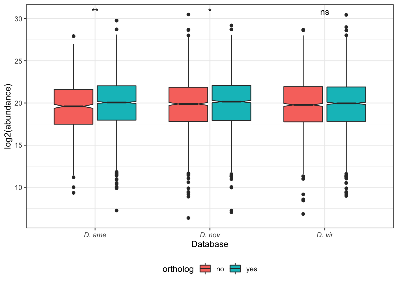
# perform KW tests
all_dat %>%
  group_by(DB) %>%
  do(fit = broom::tidy(wilcox.test(ave_abundance ~ ortholog, data = .))) %>%
  unnest(fit) %>%
  mutate(p.value = ifelse(p.value < 0.001, '< 0.001', round(p.value, 3)),
         sigLabel = case_when(p.value < 0.001 ~ "***",
                              p.value < 0.01 ~ "**",
                              p.value < 0.05 ~ "*",
                              TRUE ~ '')) %>%
  dplyr::select(-c(method:alternative)) %>%
  kable(digits = 3,
        caption = 'Wilcoxon rank sum test with continuity correction') %>%
kable_styling(full_width = FALSE)| DB | statistic | p.value | sigLabel |
|---|---|---|---|
| ame | 1113358 | 0.003 | ** |
| nov | 1469558 | 0.024 |
|
| vir | 1506247 | 0.622 |
sessionInfo()R version 4.1.3 (2022-03-10)
Platform: x86_64-apple-darwin17.0 (64-bit)
Running under: macOS Big Sur/Monterey 10.16
Matrix products: default
BLAS: /Library/Frameworks/R.framework/Versions/4.1/Resources/lib/libRblas.0.dylib
LAPACK: /Library/Frameworks/R.framework/Versions/4.1/Resources/lib/libRlapack.dylib
locale:
[1] en_GB.UTF-8/en_GB.UTF-8/en_GB.UTF-8/C/en_GB.UTF-8/en_GB.UTF-8
attached base packages:
[1] grid stats graphics grDevices utils datasets methods
[8] base
other attached packages:
[1] kableExtra_1.3.4 edgeR_3.36.0 limma_3.50.3
[4] eulerr_6.1.1 RColorBrewer_1.1-3 UpSetR_1.4.0
[7] factoextra_1.0.7 cluster_2.1.3 ggalluvial_0.12.3
[10] ComplexHeatmap_2.11.1 ggrepel_0.9.1 tidybayes_3.0.2
[13] forcats_0.5.1 stringr_1.4.0 dplyr_1.0.9
[16] purrr_0.3.4 readr_2.1.2 tidyr_1.2.0
[19] tibble_3.1.7 ggplot2_3.3.6 tidyverse_1.3.1
[22] workflowr_1.7.0
loaded via a namespace (and not attached):
[1] readxl_1.4.0 backports_1.4.1 circlize_0.4.15
[4] systemfonts_1.0.4 plyr_1.8.7 polylabelr_0.2.0
[7] svUnit_1.0.6 digest_0.6.29 foreach_1.5.2
[10] htmltools_0.5.2 viridis_0.6.2 fansi_1.0.3
[13] magrittr_2.0.3 checkmate_2.1.0 doParallel_1.0.17
[16] tzdb_0.3.0 modelr_0.1.8 matrixStats_0.62.0
[19] vroom_1.5.7 svglite_2.1.0 colorspace_2.0-3
[22] rvest_1.0.2 ggdist_3.1.1 haven_2.5.0
[25] xfun_0.31 callr_3.7.1 crayon_1.5.1
[28] jsonlite_1.8.0 iterators_1.0.14 glue_1.6.2
[31] polyclip_1.10-0 gtable_0.3.0 webshot_0.5.3
[34] GetoptLong_1.0.5 distributional_0.3.0 car_3.1-0
[37] shape_1.4.6 BiocGenerics_0.40.0 abind_1.4-5
[40] scales_1.2.0 pheatmap_1.0.12 DBI_1.1.3
[43] rstatix_0.7.0 Rcpp_1.0.9 viridisLite_0.4.0
[46] clue_0.3-61 bit_4.0.4 stats4_4.1.3
[49] MetBrewer_0.2.0 httr_1.4.3 arrayhelpers_1.1-0
[52] posterior_1.2.2 ellipsis_0.3.2 pkgconfig_2.0.3
[55] farver_2.1.1 sass_0.4.1 dbplyr_2.2.1
[58] locfit_1.5-9.6 utf8_1.2.2 reshape2_1.4.4
[61] tidyselect_1.1.2 labeling_0.4.2 rlang_1.0.4
[64] later_1.3.0 munsell_0.5.0 cellranger_1.1.0
[67] tools_4.1.3 cli_3.3.0 generics_0.1.3
[70] broom_1.0.0 evaluate_0.15 fastmap_1.1.0
[73] yaml_2.3.5 processx_3.7.0 knitr_1.39
[76] bit64_4.0.5 fs_1.5.2 whisker_0.4
[79] xml2_1.3.3 compiler_4.1.3 rstudioapi_0.13
[82] png_0.1-7 ggsignif_0.6.3 reprex_2.0.1
[85] bslib_0.3.1 stringi_1.7.8 highr_0.9
[88] ps_1.7.1 lattice_0.20-45 Matrix_1.4-1
[91] tensorA_0.36.2 vctrs_0.4.1 pillar_1.7.0
[94] lifecycle_1.0.1 jquerylib_0.1.4 GlobalOptions_0.1.2
[97] httpuv_1.6.5 R6_2.5.1 promises_1.2.0.1
[100] gridExtra_2.3 IRanges_2.28.0 codetools_0.2-18
[103] assertthat_0.2.1 rprojroot_2.0.3 rjson_0.2.21
[106] withr_2.5.0 S4Vectors_0.32.4 parallel_4.1.3
[109] hms_1.1.1 gghalves_0.1.3 coda_0.19-4
[112] rmarkdown_2.14 carData_3.0-5 Cairo_1.6-0
[115] ggpubr_0.4.0 git2r_0.30.1 getPass_0.2-2
[118] lubridate_1.8.0