Male fertility

workflowr

• Summary
• Checks
• Past versions

Last updated: 2025-04-02

Checks: 7 0

Knit directory: mito_age_fert/

This reproducible R Markdown analysis was created with workflowr (version 1.7.1). The Checks tab describes the reproducibility checks that were applied when the results were created. The Past versions tab lists the development history.

---

R Markdown file: up-to-date

Great! Since the R Markdown file has been committed to the Git repository, you know the exact version of the code that produced these results.

Environment: empty

Great job! The global environment was empty. Objects defined in the global environment can affect the analysis in your R Markdown file in unknown ways. For reproduciblity it’s best to always run the code in an empty environment.

Seed: set.seed(20230213)

The command set.seed(20230213) was run prior to running the code in the R Markdown file. Setting a seed ensures that any results that rely on randomness, e.g. subsampling or permutations, are reproducible.

Session information: recorded

Great job! Recording the operating system, R version, and package versions is critical for reproducibility.

Cache: none

Nice! There were no cached chunks for this analysis, so you can be confident that you successfully produced the results during this run.

File paths: relative

Great job! Using relative paths to the files within your workflowr project makes it easier to run your code on other machines.

Repository version: 5ebfaed

Great! You are using Git for version control. Tracking code development and connecting the code version to the results is critical for reproducibility.

The results in this page were generated with repository version 5ebfaed. See the Past versions tab to see a history of the changes made to the R Markdown and HTML files.

Note that you need to be careful to ensure that all relevant files for the analysis have been committed to Git prior to generating the results (you can use wflow_publish or wflow_git_commit). workflowr only checks the R Markdown file, but you know if there are other scripts or data files that it depends on. Below is the status of the Git repository when the results were generated:

Ignored files:
    Ignored:    .DS_Store
    Ignored:    .Rhistory
    Ignored:    .Rproj.user/
    Ignored:    analysis/.DS_Store
    Ignored:    data/.DS_Store
    Ignored:    output/.DS_Store

Untracked files:
    Untracked:  README.html
    Untracked:  check_lines.R
    Untracked:  code/data_wrangling.R
    Untracked:  code/female_predictions_13-Feb-2025.sh
    Untracked:  code/female_rate_predictions.R
    Untracked:  code/plotting_Script.R
    Untracked:  data/Data_raw_emmely.csv
    Untracked:  data/SNP_data/
    Untracked:  data/defence.csv
    Untracked:  data/male_fertility.csv
    Untracked:  data/mito_34sigdiffSNPs_consensus_incl_colnames.csv
    Untracked:  data/mito_mt_copy_number.xlsx
    Untracked:  data/mito_mt_seq_major_alleles_sig_snptable.csv
    Untracked:  data/mito_mt_seq_sig_annotated.csv
    Untracked:  data/mito_mt_seq_sig_annotated.vcf
    Untracked:  data/offence.csv
    Untracked:  data/rawdata_PCA.csv
    Untracked:  data/snp-gene.txt
    Untracked:  data/sperm_metabolic_rate.csv
    Untracked:  data/sperm_viability.csv
    Untracked:  data/wrangled/
    Untracked:  figures/
    Untracked:  output/SNP_clusters.csv
    Untracked:  output/anova_tables/
    Untracked:  output/bod_brm.rds
    Untracked:  output/female_rate_dredge.rds
    Untracked:  output/female_rates_bb.Rdata
    Untracked:  output/female_rates_boot.Rdata
    Untracked:  output/female_rates_poly.Rdata
    Untracked:  output/fst_tabs.csv
    Untracked:  output/male_fec_dredge.rds
    Untracked:  output/male_hatch_dredge.rds
    Untracked:  output/male_hatch_dredge_reduced.rds
    Untracked:  output/sperm_met_dredge.rds
    Untracked:  output/viab_ctrl_dredge.rds
    Untracked:  output/viab_trt_dredge.rds
    Untracked:  snp_matrix_dobler.csv

Unstaged changes:
    Modified:   analysis/SNP_clusters.Rmd
    Deleted:    analysis/sperm_comp.Rmd
    Modified:   data/README.md

Note that any generated files, e.g. HTML, png, CSS, etc., are not included in this status report because it is ok for generated content to have uncommitted changes.

---

These are the previous versions of the repository in which changes were made to the R Markdown (analysis/male_fertility.Rmd) and HTML (docs/male_fertility.html) files. If you’ve configured a remote Git repository (see ?wflow_git_remote), click on the hyperlinks in the table below to view the files as they were in that past version.

File	Version	Author	Date	Message
Rmd	5ebfaed	MartinGarlovsky	2025-04-02	wflow_publish(c("analysis/body_size.Rmd", "analysis/female_fertility.Rmd",
html	0ffce9c	MartinGarlovsky	2024-10-10	Build site.
Rmd	dfaa300	MartinGarlovsky	2024-10-10	wflow_publish("analysis/male_fertility.Rmd")
html	a7bae31	MartinGarlovsky	2024-10-09	Build site.
Rmd	5f3a2a7	MartinGarlovsky	2024-10-09	wflow_publish("analysis/male_fertility.Rmd")

---

Load packages

library(tidyverse)

library(lme4)
library(DHARMa)
library(emmeans)
library(kableExtra)
library(knitrhooks) # install with devtools::install_github("nathaneastwood/knitrhooks")
library(showtext)

library(conflicted)

select <- dplyr::select
filter <- dplyr::filter

output_max_height() # a knitrhook option

options(stringsAsFactors = FALSE)

# colour palettes
met.pal <- MetBrewer::met.brewer('Johnson')
met3 <- met.pal[c(1, 3, 5)]

# set contrasts
options(contrasts = c("contr.sum", "contr.poly"))

Load data

# fecundity and hatching success
male_fert_filt <- read.csv('data/wrangled/male_fertility.csv') %>% 
  mutate(age = fct_relevel(age, c("young","old")),
         mito_snp = as.factor(mito_snp),
         coevolved = if_else(mito == nuclear, "matched", "mismatched"))

#xtabs(~ mito + nuclear, data = male_fert)

# sperm viability
sperm_vib_filt <- read.csv("data/wrangled/sperm_viability_wrangled.csv") %>% 
  mutate(age = fct_relevel(age, c("young","old")),
         mito_snp = as.factor(mito_snp),
         coevolved = if_else(mito == nuclear, "matched", "mismatched"))

#xtabs(~ mito + nuclear, data = sperm_vib_filt)

# sperm metabolism
sperm_met <- read.csv("data/wrangled/sperm_met_wrangled.csv") %>% 
  mutate(age = fct_relevel(age, c("young","old")),
         mito_snp = as.factor(mito_snp),
         p.a2 = a2/100, # convert to percentage proportion
         coevolved = if_else(mito == nuclear, "matched", "mismatched")) 

#xtabs(~ mito + nuclear, data = sperm_met)

# sperm competition data
## P1
defence <- read.csv("data/wrangled/sperm_defence.csv", header = TRUE) %>% 
  mutate(mito_snp = as.factor(mito_snp),
         Day = ordered(Day),
         coevolved = if_else(mito == nuclear, "matched", "mismatched"))

## P2
offence <- read.csv("data/wrangled/sperm_offence.csv", header = TRUE) %>% 
  mutate(mito_snp = as.factor(mito_snp),
         Day = ordered(Day),
         coevolved = if_else(mito == nuclear, "matched", "mismatched"))

> Fecundity

male_fert_filt %>% 
  group_by(mito, nuclear, age) %>% 
  summarise(mn = mean(total_eggs),
            se = sd(total_eggs)/sqrt(n()),
            s95 = se * 1.96) %>% 
  ggplot(aes(x = mito, y = mn, fill = nuclear)) +
  geom_point(data = male_fert_filt,
             aes(y = total_eggs, colour = nuclear), alpha = .25,
             position = position_jitterdodge(dodge.width = .5, jitter.width = .1)) +
  geom_errorbar(aes(ymin = mn - s95, ymax = mn + s95), 
                width = .25, position = position_dodge(width = .5)) +
  geom_point(size = 3, pch = 21, position = position_dodge(width = .5)) +
  labs(y = 'Partner fecundity') +
  facet_wrap(~ age, scales = 'free_x') +
  scale_colour_manual(values = met3) +
  scale_fill_manual(values = met3) +
  theme_bw() + 
  theme() + 
  NULL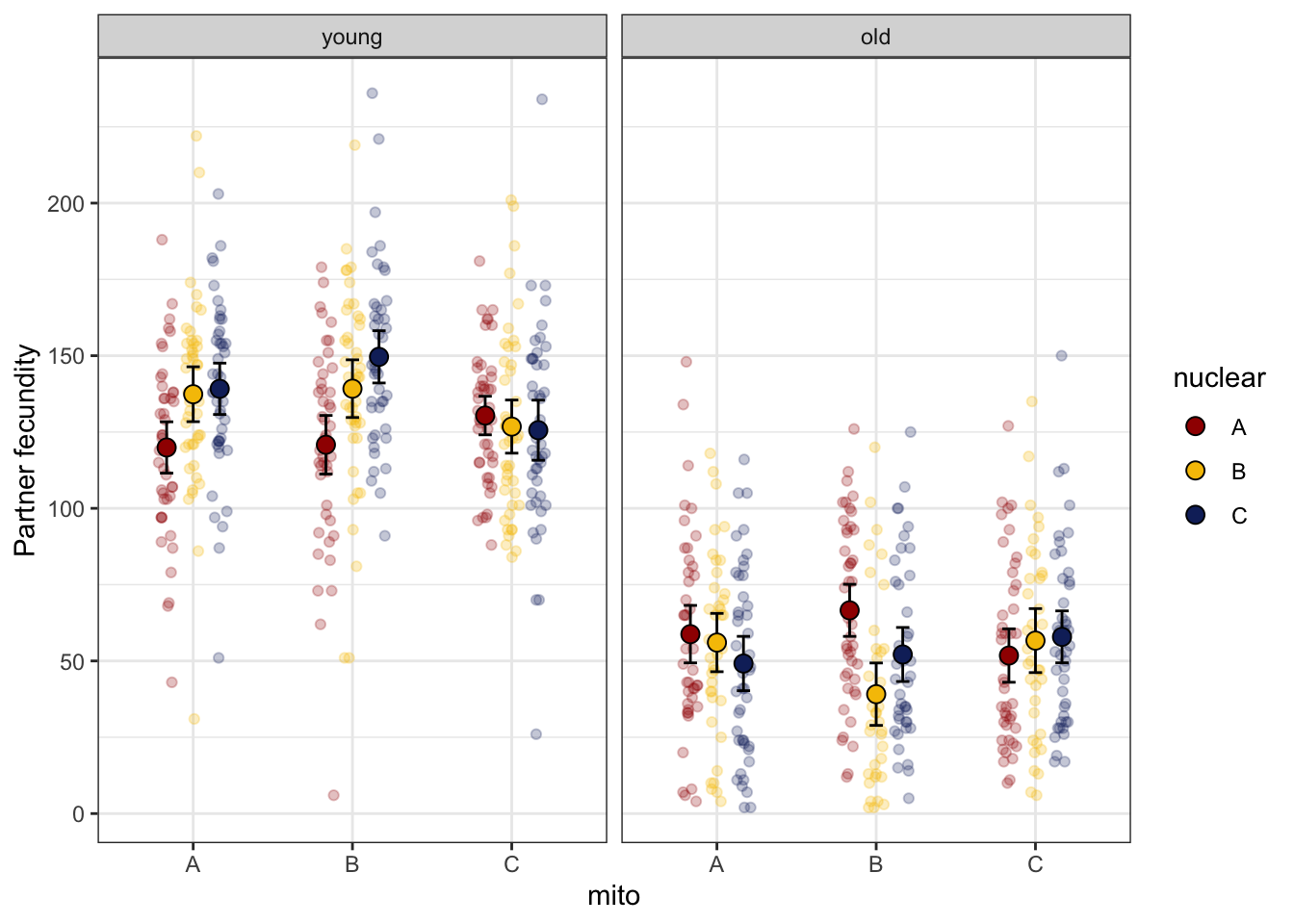

Past versions of unnamed-chunk-3-1.png

Version	Author	Date
a7bae31	MartinGarlovsky	2024-10-09

hist(male_fert_filt$total_eggs, breaks = 50)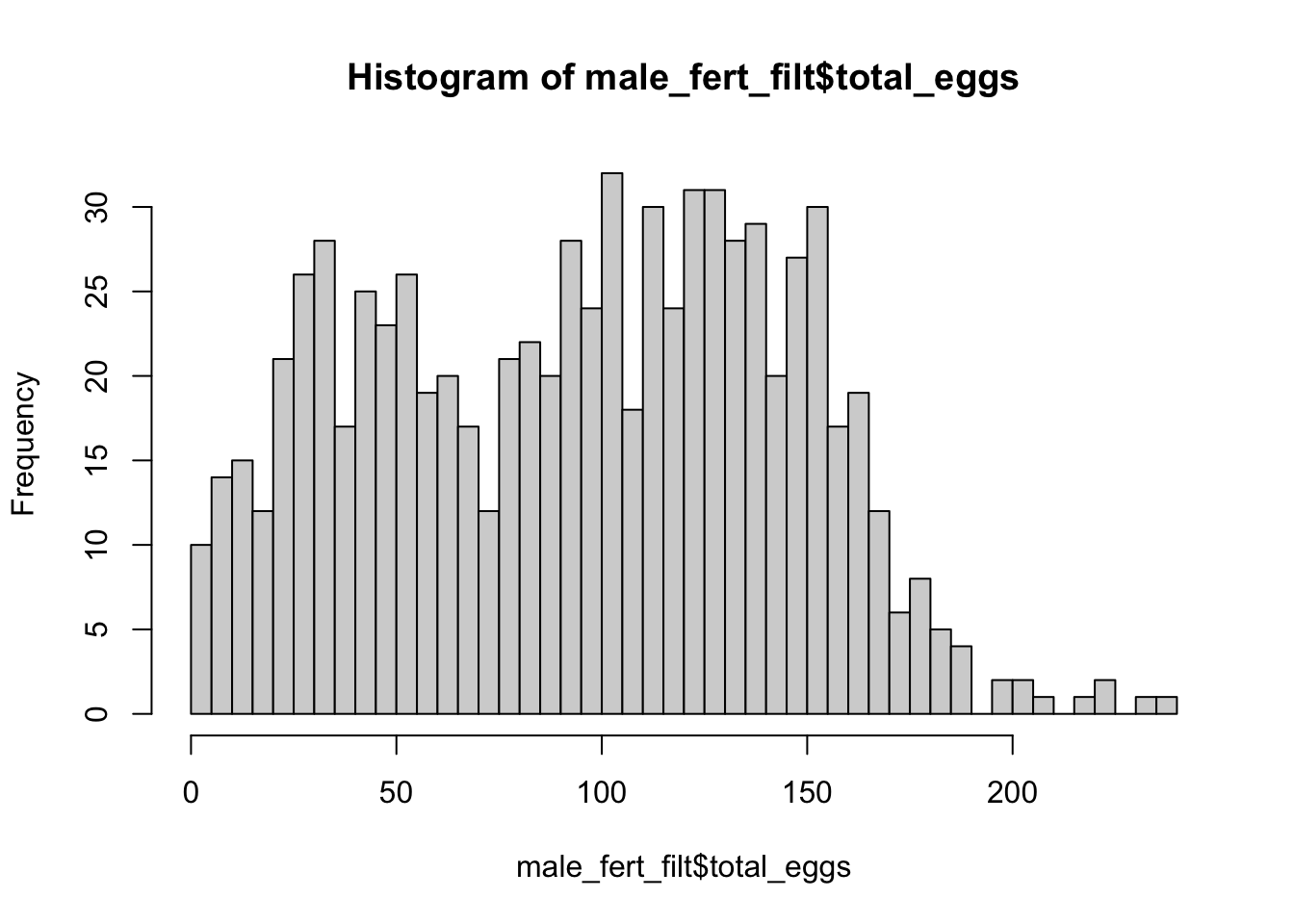

Past versions of unnamed-chunk-3-2.png

Version	Author	Date
a7bae31	MartinGarlovsky	2024-10-09

# fit linear model - model diagnostics look better?
male_fec_test <- lmerTest::lmer(total_eggs ~ mito * nuclear * age + (1|LINE:age), 
                                data = male_fert_filt, REML = TRUE) 

anova(male_fec_test, type = "III", ddf = "Kenward-Roger") %>% 
  broom::tidy() %>% 
  as_tibble() %>% #write_csv("output/anova_tables/male_fecundity.csv") %>% # save anova table for supp. tables
  kable(digits = 3, 
        caption = 'Type III Analysis of Variance Table with Kenward-Roger`s method') %>% 
  kable_styling(full_width = FALSE)

Type III Analysis of Variance Table with Kenward-Roger`s method

term	sumsq	meansq	NumDF	DenDF	statistic	p.value
mito	655.057	327.529	2	36.119	0.375	0.690
nuclear	1328.203	664.101	2	36.089	0.761	0.474
age	628683.021	628683.021	1	36.120	720.654	0.000
mito:nuclear	3177.393	794.348	4	36.089	0.911	0.468
mito:age	2413.910	1206.955	2	36.119	1.384	0.264
nuclear:age	9125.522	4562.761	2	36.089	5.230	0.010
mito:nuclear:age	12241.283	3060.321	4	36.089	3.508	0.016

#summary(male_fec_test)

fec_emm <- emmeans(male_fec_test, ~ mito * nuclear * age)

#pairs(fec_emm, simple = list("age", "mito", "nuclear"))

bind_rows(pairs(fec_emm, simple = list("age", "mito", "nuclear"))$`simple contrasts for age` %>% broom::tidy(),
          pairs(fec_emm, simple = list("age", "mito", "nuclear"))$`simple contrasts for mito` %>% broom::tidy() %>%
            rename(p.value = adj.p.value),
          pairs(fec_emm, simple = list("age", "mito", "nuclear"))$`simple contrasts for nuclear` %>% broom::tidy() %>%
            rename(p.value = adj.p.value)) %>% 
  mutate(p.val = ifelse(p.value < 0.001, '< 0.001', round(p.value, 3))) %>% 
  select(-p.value, -term) %>% relocate(age, .before = contrast) %>% 
  kable(digits = 3, 
        caption = 'Posthoc Tukey tests to compare which groups differ') %>% 
  kable_styling(full_width = FALSE) %>%
  kableExtra::group_rows("Age", 1, 9) %>%
  kableExtra::group_rows("Mito contrasts", 10, 27) %>%
  kableExtra::group_rows("Nuclear contrasts", 28, 45)

Posthoc Tukey tests to compare which groups differ

mito	nuclear	age	contrast	null.value	estimate	std.error	df	statistic	p.val
Age
A	A	NA	young - old	0	61.156	8.602	34.548	7.109	< 0.001
B	A	NA	young - old	0	54.244	8.602	34.548	6.306	< 0.001
C	A	NA	young - old	0	78.724	8.628	34.960	9.124	< 0.001
A	B	NA	young - old	0	81.208	8.825	37.887	9.202	< 0.001
B	B	NA	young - old	0	100.156	8.882	39.205	11.276	< 0.001
C	B	NA	young - old	0	70.090	8.888	39.184	7.886	< 0.001
A	C	NA	young - old	0	90.000	8.602	34.548	10.463	< 0.001
B	C	NA	young - old	0	97.573	8.684	35.849	11.236	< 0.001
C	C	NA	young - old	0	67.711	8.602	34.548	7.871	< 0.001
Mito contrasts
NA	A	young	A - B	0	-0.889	8.602	34.548	-0.103	0.994
NA	A	young	A - C	0	-10.467	8.602	34.548	-1.217	0.452
NA	A	young	B - C	0	-9.578	8.602	34.548	-1.113	0.512
NA	B	young	A - B	0	-1.822	8.602	34.548	-0.212	0.976
NA	B	young	A - C	0	10.600	8.602	34.548	1.232	0.443
NA	B	young	B - C	0	12.422	8.602	34.548	1.444	0.33
NA	C	young	A - B	0	-10.467	8.602	34.548	-1.217	0.452
NA	C	young	A - C	0	13.556	8.602	34.548	1.576	0.269
NA	C	young	B - C	0	24.022	8.602	34.548	2.793	0.022
NA	A	old	A - B	0	-7.800	8.602	34.548	-0.907	0.64
NA	A	old	A - C	0	7.102	8.628	34.960	0.823	0.691
NA	A	old	B - C	0	14.902	8.628	34.960	1.727	0.21
NA	B	old	A - B	0	17.126	9.098	42.719	1.882	0.156
NA	B	old	A - C	0	-0.517	9.104	42.692	-0.057	0.998
NA	B	old	B - C	0	-17.643	9.160	44.100	-1.926	0.143
NA	C	old	A - B	0	-2.894	8.684	35.849	-0.333	0.941
NA	C	old	A - C	0	-8.733	8.602	34.548	-1.015	0.572
NA	C	old	B - C	0	-5.839	8.684	35.849	-0.672	0.781
Nuclear contrasts
A	NA	young	A - B	0	-17.444	8.602	34.548	-2.028	0.121
A	NA	young	A - C	0	-19.222	8.602	34.548	-2.235	0.079
A	NA	young	B - C	0	-1.778	8.602	34.548	-0.207	0.977
B	NA	young	A - B	0	-18.378	8.602	34.548	-2.136	0.097
B	NA	young	A - C	0	-28.800	8.602	34.548	-3.348	0.005
B	NA	young	B - C	0	-10.422	8.602	34.548	-1.212	0.454
C	NA	young	A - B	0	3.622	8.602	34.548	0.421	0.907
C	NA	young	A - C	0	4.800	8.602	34.548	0.558	0.843
C	NA	young	B - C	0	1.178	8.602	34.548	0.137	0.99
A	NA	old	A - B	0	2.608	8.825	37.887	0.295	0.953
A	NA	old	A - C	0	9.622	8.602	34.548	1.119	0.509
A	NA	old	B - C	0	7.015	8.825	37.887	0.795	0.708
B	NA	old	A - B	0	27.533	8.882	39.205	3.100	0.01
B	NA	old	A - C	0	14.528	8.684	35.849	1.673	0.229
B	NA	old	B - C	0	-13.005	8.962	40.582	-1.451	0.325
C	NA	old	A - B	0	-5.012	8.913	39.619	-0.562	0.841
C	NA	old	A - C	0	-6.213	8.628	34.960	-0.720	0.753
C	NA	old	B - C	0	-1.201	8.888	39.184	-0.135	0.99

>>> Results

>>>> Reaction norms

# reaction norms
male_fecundity_norm <- emmeans(male_fec_test, ~ mito * nuclear * age) %>% as_tibble() %>% 
  ggplot(aes(x = nuclear, y = emmean, fill = mito)) +
  geom_line(aes(group = mito, colour = mito), position = position_dodge(width = .5)) +
  # geom_errorbar(aes(ymin = lower.CL, ymax = upper.CL), 
  #               width = .25, position = position_dodge(width = .5)) +
  geom_point(size = 3, pch = 21, position = position_dodge(width = .5)) +
  labs(y = 'Partner fecundity (EMM ± 95% CI)') +
  scale_colour_manual(values = met3) +
  scale_fill_manual(values = met3) +
  facet_wrap(~ age) +
  theme_bw() + 
  theme() +
  NULL

male_fecundity_norm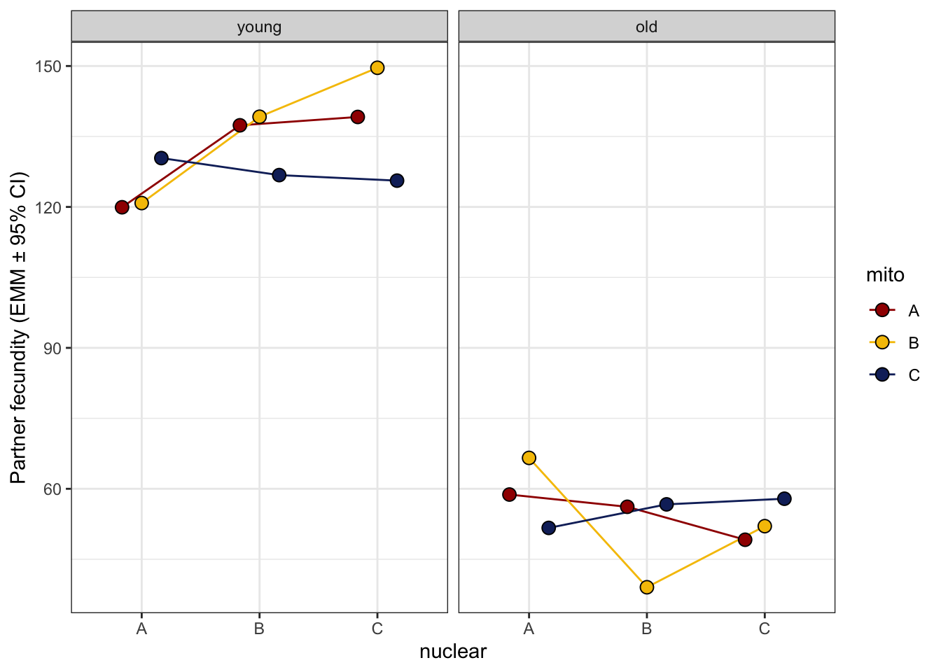

Past versions of unnamed-chunk-4-1.png

Version	Author	Date
a7bae31	MartinGarlovsky	2024-10-09

>>>> Raw data

male_fecundity_raw <- emmeans(male_fec_test, ~ mito * nuclear * age) %>% as_tibble() %>% 
  ggplot(aes(x = nuclear, y = emmean, fill = mito)) +
  geom_jitter(data = male_fert_filt,
              aes(y = total_eggs, colour = mito),
               position = position_jitterdodge(dodge.width = .5, jitter.width = .1),
              size = 0.75, alpha = .1) +
  geom_jitter(data = male_fert_filt %>% 
                group_by(LINE, age) %>% 
                summarise(mn = mean(total_eggs)) %>% 
                separate(LINE, into = c("mito", "nuclear", NA), sep = "(?<=.)", remove = FALSE),
              aes(y = mn, colour = mito),
              position = position_jitterdodge(dodge.width = .5, jitter.width = .1),
              alpha = .85, size = 2) +
  geom_errorbar(aes(ymin = lower.CL, ymax = upper.CL), 
                width = .25, position = position_dodge(width = .5)) +
  geom_point(size = 3, pch = 21, position = position_dodge(width = .5)) +
  labs(y = 'Partner fecundity (EMM ± 95% CIs)') +
  scale_colour_manual(values = met3) +
  scale_fill_manual(values = met3) +
  facet_wrap(~ age) +
  theme_bw() + 
  theme() + 
  geom_text(data = male_fert_filt %>% group_by(mito, nuclear, age) %>% count(), aes(y = -5, label = n), 
            size = 2, position = position_dodge(width = .5)) + 
  #ggsave('figures/male_fecundity_raw.pdf', height = 4, width = 8, dpi = 600, useDingbats = FALSE) +
  NULL

male_fecundity_raw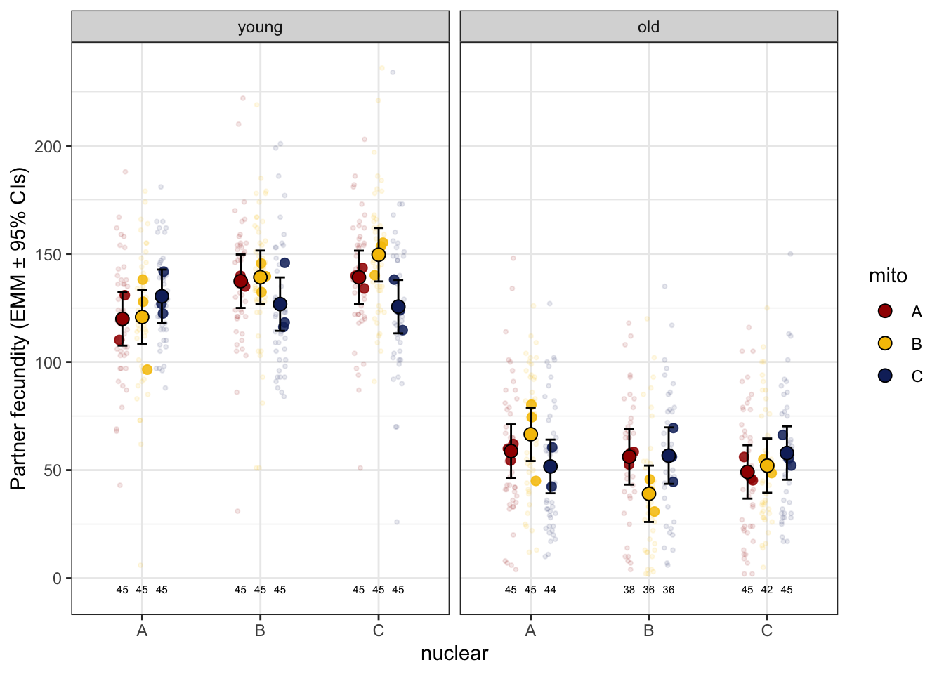

Past versions of unnamed-chunk-5-1.png

Version	Author	Date
a7bae31	MartinGarlovsky	2024-10-09

>>> Matched vs. mismatched

male_fec_coevo <- lmerTest::lmer(total_eggs ~ coevolved * age + (1 + age|LINE), 
                                 data = male_fert_filt, REML = TRUE) 

anova(male_fec_coevo, type = "III", ddf = "Kenward-Roger") %>% 
  broom::tidy() %>% 
  as_tibble()

# A tibble: 3 × 7
  term            sumsq  meansq NumDF DenDF statistic  p.value
                           
1 coevolved       1256.   1256.     1  24.9     1.44  2.42e- 1
2 age           442492. 442492.     1  24.9   507.    4.32e-18
3 coevolved:age    151.    151.     1  24.9     0.173 6.81e- 1

#summary(male_fec_coevo)

>>> Mito-type analysis

# fit linear model
male_fec1_snp <- lmerTest::lmer(total_eggs ~ mito_snp * nuclear * age + (1|LINE:age), 
                                data = male_fert_filt, REML = TRUE) 

anova(male_fec1_snp, type = "III", ddf = "Kenward-Roger") %>% broom::tidy() %>% 
  as_tibble() %>% 
  kable(digits = 3, 
        caption = 'Type III Analysis of Variance Table with Kenward-Roger`s method') %>% 
  kable_styling(full_width = FALSE)

Type III Analysis of Variance Table with Kenward-Roger`s method

term	sumsq	meansq	NumDF	DenDF	statistic	p.value
mito_snp	1680.257	210.032	8	17.998	0.241	0.977
nuclear	169.779	84.889	2	18.050	0.097	0.908
age	254992.935	254992.935	1	17.837	292.215	0.000
mito_snp:nuclear	4216.698	602.385	7	18.144	0.690	0.679
mito_snp:age	3795.329	474.416	8	17.998	0.544	0.809
nuclear:age	5043.513	2521.757	2	18.050	2.890	0.082
mito_snp:nuclear:age	4183.266	597.609	7	18.144	0.685	0.683

#car::Anova(male_fec1_snp, type = "III")

fec_emm_snp <- emmeans(male_fec1_snp, ~ mito_snp * nuclear * age)

male_fecundity_snp <- fec_emm_snp %>% as_tibble() %>% drop_na() %>% 
  ggplot(aes(x = nuclear, y = emmean, fill = mito_snp)) +
  geom_jitter(data = male_fert_filt,
              aes(y = total_eggs, colour = mito_snp),
               position = position_jitterdodge(dodge.width = .5, jitter.width = .1),
              alpha = .25) + 
  geom_errorbar(aes(ymin = lower.CL, ymax = upper.CL), 
                width = .25, position = position_dodge(width = .5)) +
  geom_point(size = 3, pch = 21, position = position_dodge(width = .5)) +
  labs(y = 'Partner fecundity (EMM ± 95% CIs)') +
  facet_wrap(~ age) +
  scale_colour_viridis_d(option = "H") +
  scale_fill_viridis_d(option = "H") +
  theme_bw() + 
  theme() + 
  #ggsave('figures/male_fecundity_snp.pdf', height = 4, width = 8.5, dpi = 600, useDingbats = FALSE) +
  NULL

male_fecundity_snp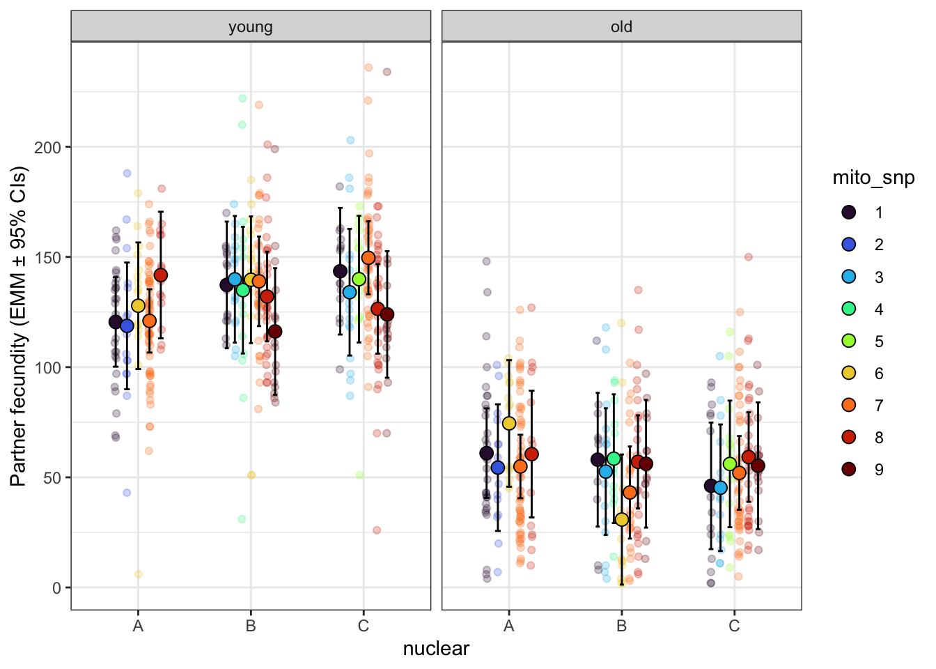

Past versions of unnamed-chunk-7-1.png

Version	Author	Date
a7bae31	MartinGarlovsky	2024-10-09

> Hatching success

Hatching success, our proxy for fertilisation success, shows different patterns in young and old males. In old males there is a very bimodal distribtuion, i.e., some males are fertile while others are completely sterile. Therefore, we model young and old males separately.

male_fert_filt %>%
  group_by(mito, nuclear, age) %>% 
  summarise(mn = mean(fertilised),
            se = sd(fertilised)/sqrt(n()),
            s95 = se * 1.96) %>% 
  ggplot(aes(x = nuclear, y = mn, fill = mito)) +
  geom_point(data = male_fert_filt,
             aes(y = fertilised, colour = mito), alpha = .25,
             position = position_jitterdodge(dodge.width = .5, jitter.width = .1)) +
  geom_errorbar(aes(ymin = mn - s95, ymax = mn + s95), 
                width = .25, position = position_dodge(width = .5)) +
  geom_point(size = 3, pch = 21, position = position_dodge(width = .5)) +
  labs(y = 'Hatching success') +
  coord_cartesian(ylim = c(0, 1)) +
  facet_wrap(~ age, scales = 'free_x') +
  scale_colour_manual(values = met3) +
  scale_fill_manual(values = met3) +
  theme_bw() + 
  theme() + 
  #ggsave('figures/male_hatchingsuccess_all.pdf', height = 4, width = 9, dpi = 600, useDingbats = FALSE) +
  NULL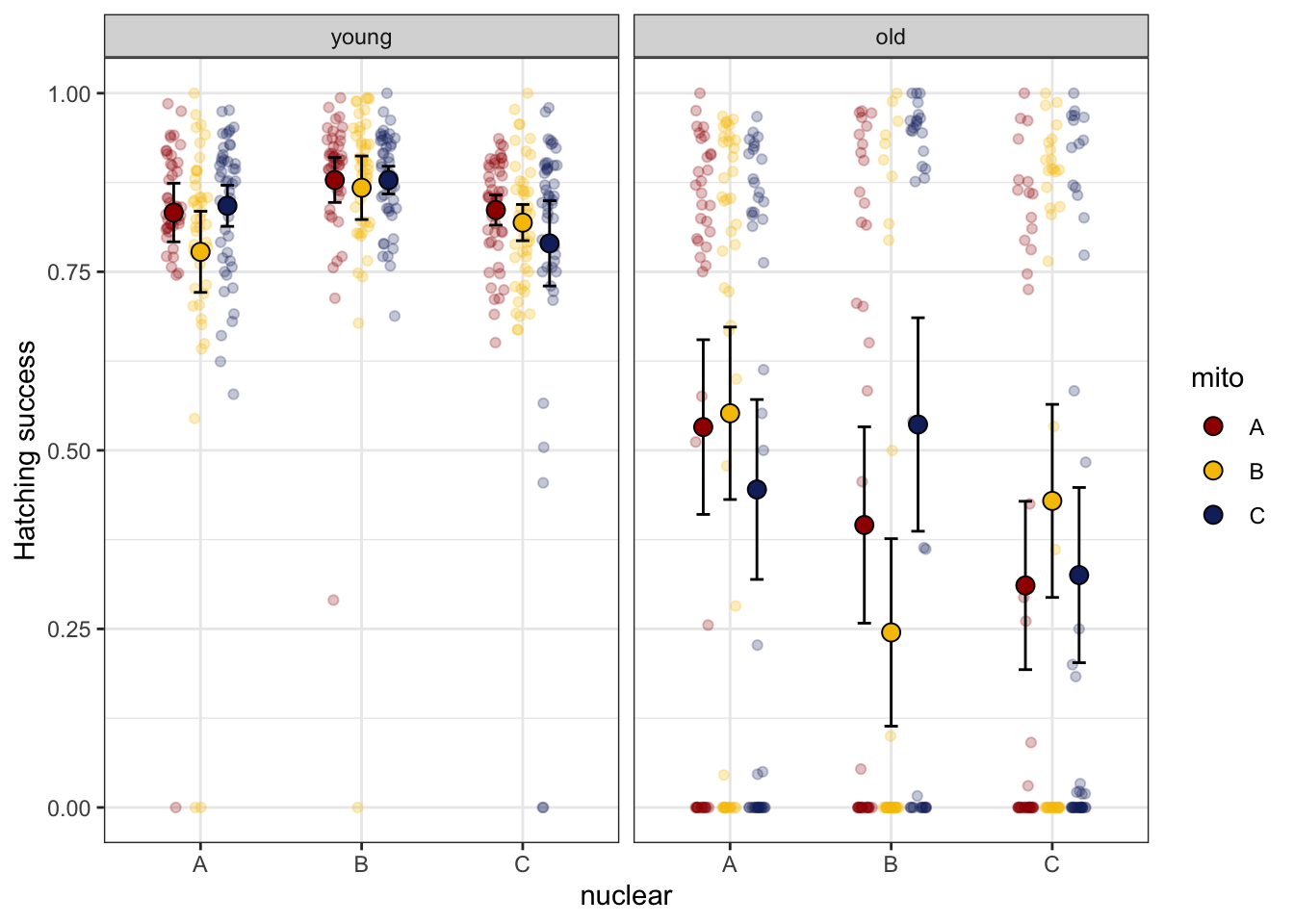

Past versions of unnamed-chunk-8-1.png

Version	Author	Date
a7bae31	MartinGarlovsky	2024-10-09

#xtabs(~ mtn + age, data = male_fert_filt)

>>> Young males

In young males we model the proportion of eggs that hatch.

##model young only
hatch2 <- glmer(cbind(total_offs, total_fail) ~ mito * nuclear + (1|LINE) + (1|OLRE),
                data = male_fert_filt %>% filter(age == "young"), 
                family = 'binomial')

>>>> Check model diagnostics

performance::check_model(hatch2)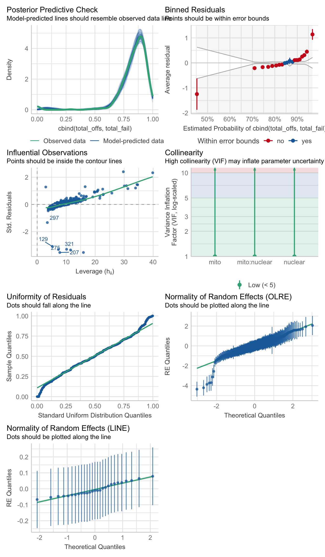

Past versions of unnamed-chunk-10-1.png

Version	Author	Date
0ffce9c	MartinGarlovsky	2024-10-10
a7bae31	MartinGarlovsky	2024-10-09

performance::check_overdispersion(hatch2)

# Overdispersion test

 dispersion ratio = 1.020
          p-value = 0.688

testDispersion(hatch2)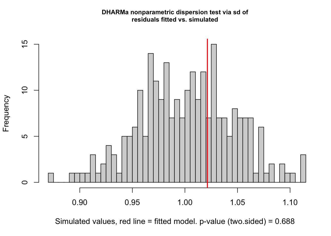

Past versions of unnamed-chunk-11-1.png

Version	Author	Date
a7bae31	MartinGarlovsky	2024-10-09

    DHARMa nonparametric dispersion test via sd of residuals fitted vs.
    simulated

data:  simulationOutput
dispersion = 1.02, p-value = 0.688
alternative hypothesis: two.sided

simulationOutput <- simulateResiduals(fittedModel = hatch2, plot = FALSE)
hist(residuals(simulationOutput))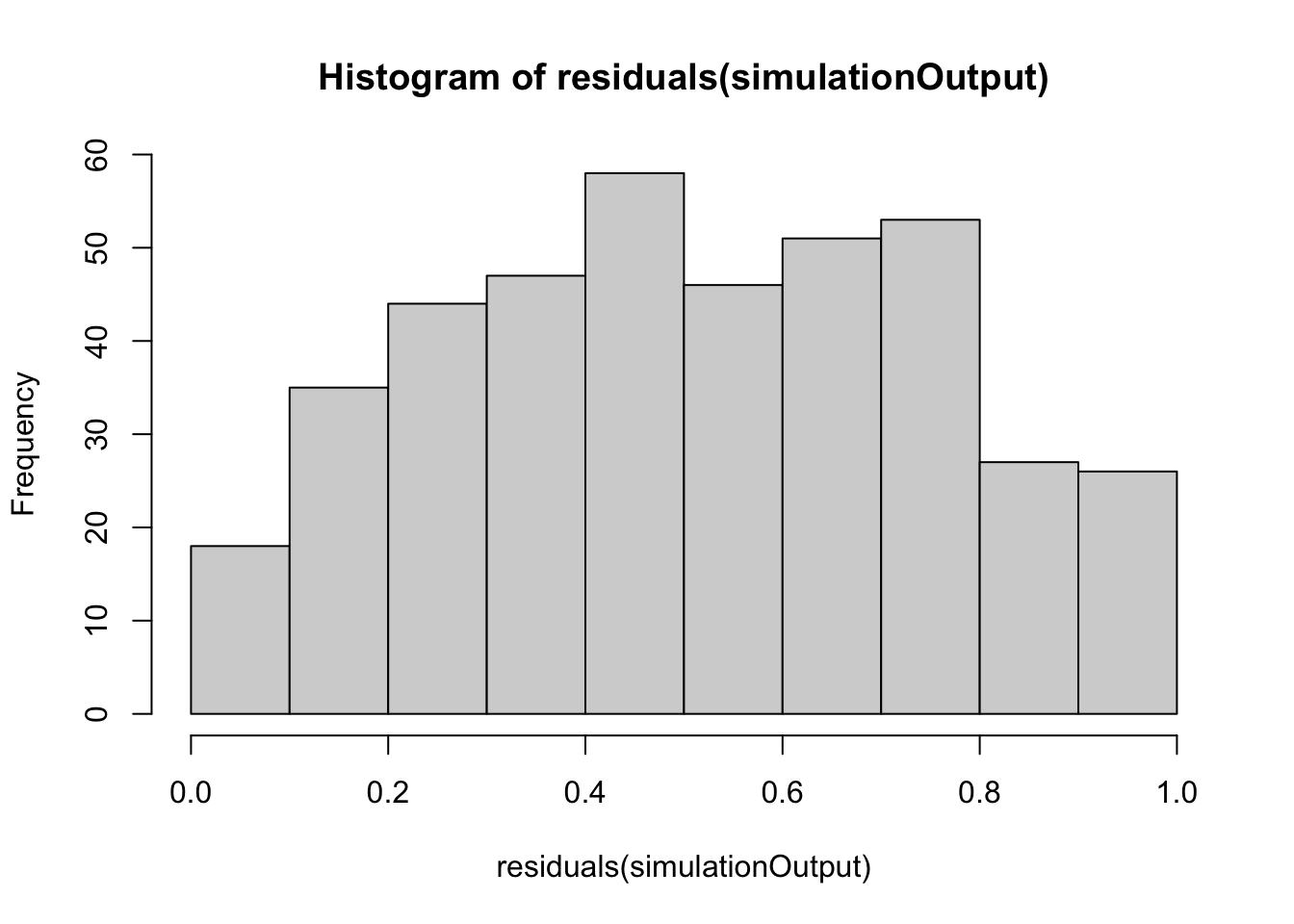

Past versions of unnamed-chunk-11-2.png

Version	Author	Date
a7bae31	MartinGarlovsky	2024-10-09

hist(residuals(simulationOutput, quantileFunction = qnorm, outlierValues = c(-7,7)), breaks = 50)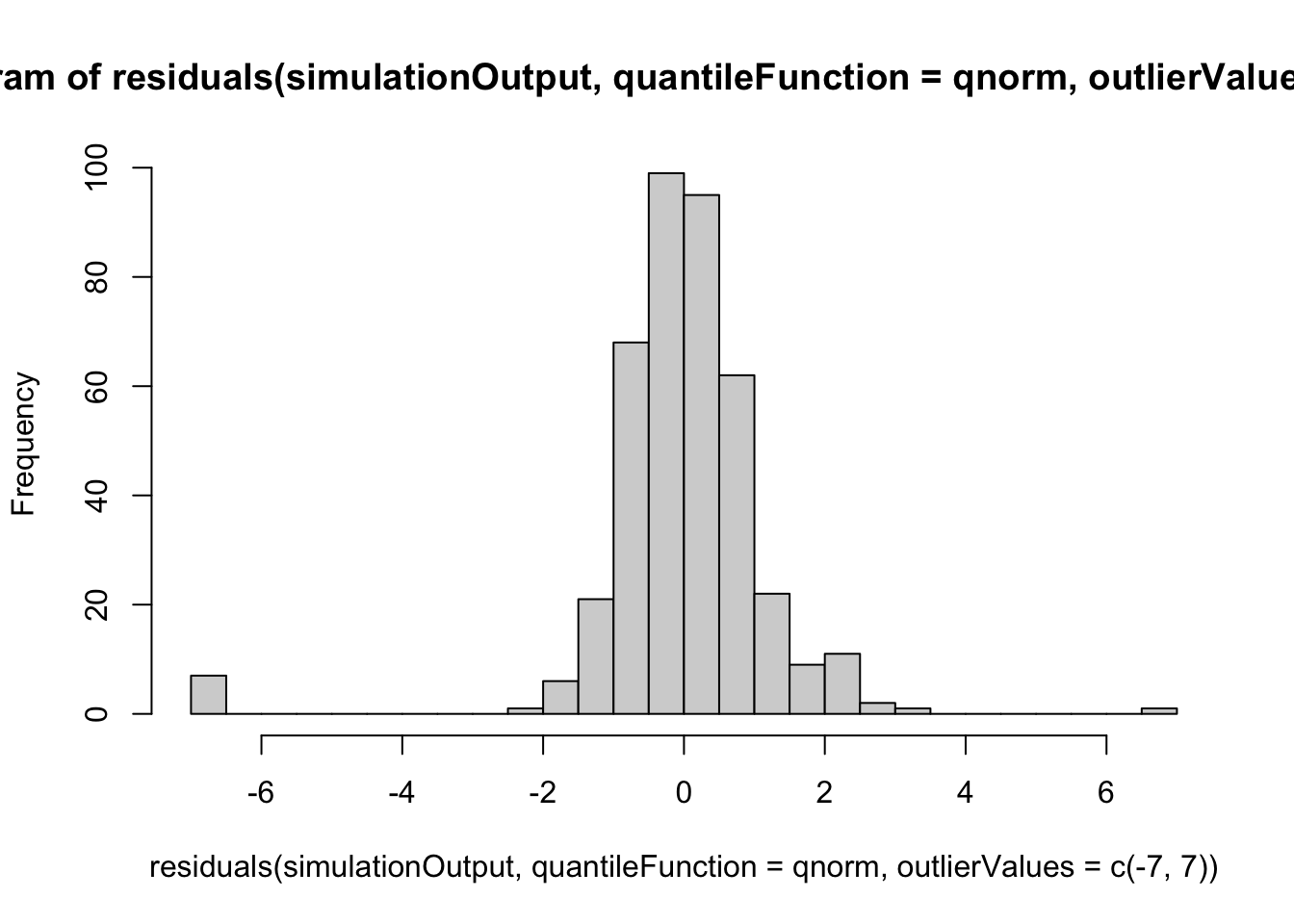

Past versions of unnamed-chunk-11-3.png

Version	Author	Date
a7bae31	MartinGarlovsky	2024-10-09

plot(simulationOutput)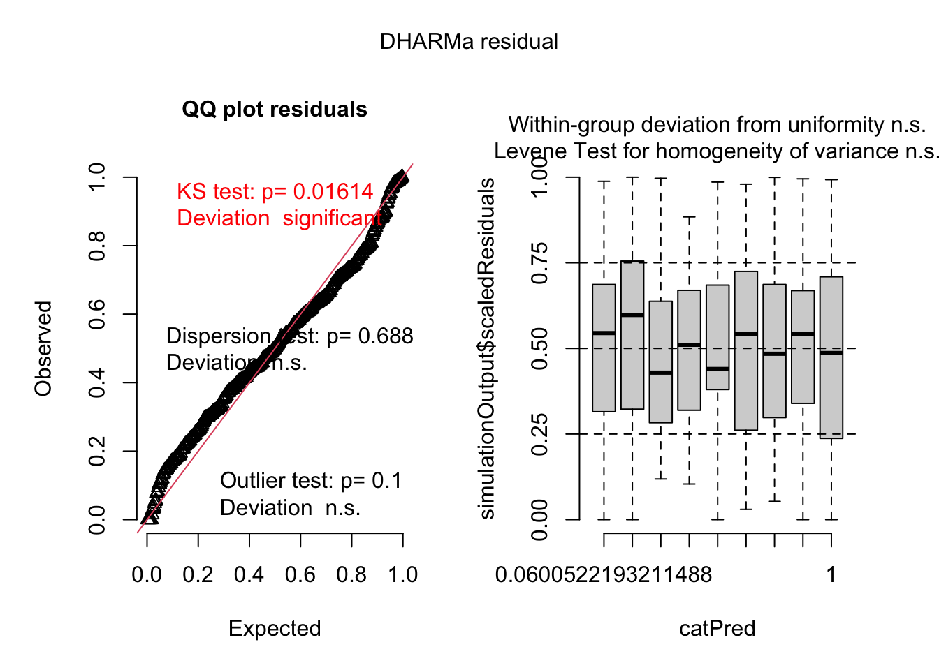

Past versions of unnamed-chunk-11-4.png

Version	Author	Date
a7bae31	MartinGarlovsky	2024-10-09

>>> Results

car::Anova(hatch2, type = "3") %>% 
  broom::tidy() %>% 
  as_tibble() %>% #write_csv("output/anova_tables/male_fert_young.csv") %>% # save anova table for supp. tables
  kable(digits = 3, 
        caption = 'Analysis of Deviance Table (Type III Wald chisquare tests)') %>% 
  kable_styling(full_width = FALSE)

Analysis of Deviance Table (Type III Wald chisquare tests)

term	statistic	df	p.value
(Intercept)	1422.684	1	0.000
mito	1.540	2	0.463
nuclear	26.190	2	0.000
mito:nuclear	5.198	4	0.268

#summary(hatch2)

hatch_emm2 <- emmeans(hatch2, ~ mito * nuclear)

emmeans(hatch2, pairwise ~ nuclear, adjust = "tukey")$contrasts %>% as_tibble() %>% 
  kable(digits = 3, 
        caption = 'Posthoc Tukey tests for comparison between nuclear genotypes') %>% 
  kable_styling(full_width = FALSE)

Posthoc Tukey tests for comparison between nuclear genotypes

contrast	estimate	SE	df	z.ratio	p.value
A - B	-0.514	0.119	Inf	-4.310	0.000
A - C	0.028	0.118	Inf	0.239	0.969
B - C	0.542	0.119	Inf	4.563	0.000

>>>> Reaction norms

# reaction norms
hatchingsuccess_young_norm <- emmeans(hatch2, ~ mito * nuclear, type = 'response') %>% as_tibble() %>% 
  ggplot(aes(x = nuclear, y = prob, fill = mito)) +
  geom_line(aes(group = mito, colour = mito), position = position_dodge(width = .5)) +
  geom_point(size = 3, pch = 21, position = position_dodge(width = .5)) +
  labs(y = '% Hatching success (EMM ± 95% CI)') +
  scale_colour_manual(values = met3) +
  scale_fill_manual(values = met3) +
  theme_bw() + 
  theme() +
  NULL

hatchingsuccess_young_norm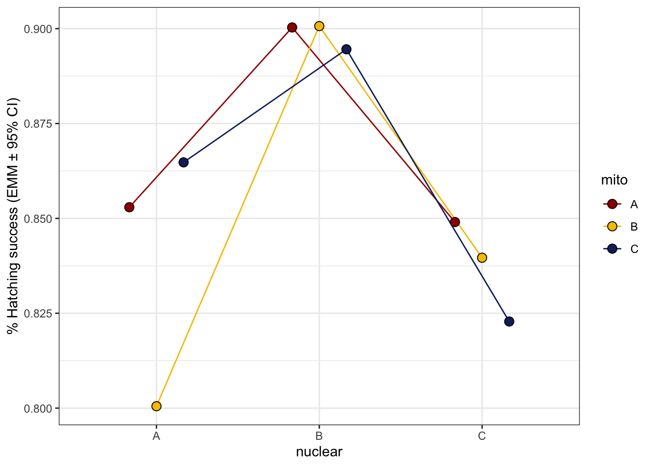

Past versions of unnamed-chunk-13-1.png

Version	Author	Date
a7bae31	MartinGarlovsky	2024-10-09

>>>> Raw data with means

hatchingsuccess_young_raw <- emmeans(hatch2, ~ mito * nuclear, type = 'response') %>% as_tibble() %>% 
  ggplot(aes(x = nuclear, y = prob, fill = mito)) +
  geom_jitter(data = male_fert_filt %>% filter(age == "young"),
              aes(y = fertilised, colour = mito),
               position = position_jitterdodge(dodge.width = .5, jitter.width = .1),
              alpha = .25) + 
  geom_jitter(data = male_fert_filt %>% filter(age == "young") %>% 
                group_by(LINE, age) %>% 
                summarise(mn = mean(fertilised)) %>% 
                separate(LINE, into = c("mito", "nuclear", NA), sep = "(?<=.)", remove = FALSE),
              aes(y = mn, colour = mito),
              position = position_jitterdodge(dodge.width = .5, jitter.width = .1),
              alpha = .85, size = 2) +
  geom_errorbar(aes(ymin = asymp.LCL, ymax = asymp.UCL), 
                width = .25, position = position_dodge(width = .5)) +
  geom_point(size = 3, pch = 21, position = position_dodge(width = .5)) +
  labs(y = '% Hatching success (EMM ± 95% CIs)') +
  scale_colour_manual(values = met3) +
  scale_fill_manual(values = met3) +
  theme_bw() + 
  theme() + 
  geom_text(data = male_fert_filt %>% filter(age == "young") %>% 
              group_by(mito, nuclear) %>% count(), aes(y = -0.04, label = n), 
            size = 2, position = position_dodge(width = .5)) + 
  #ggsave('figures/hatchingsuccess_young_raw.pdf', height = 4, width = 5, dpi = 600, useDingbats = FALSE) +
  NULL

hatchingsuccess_young_raw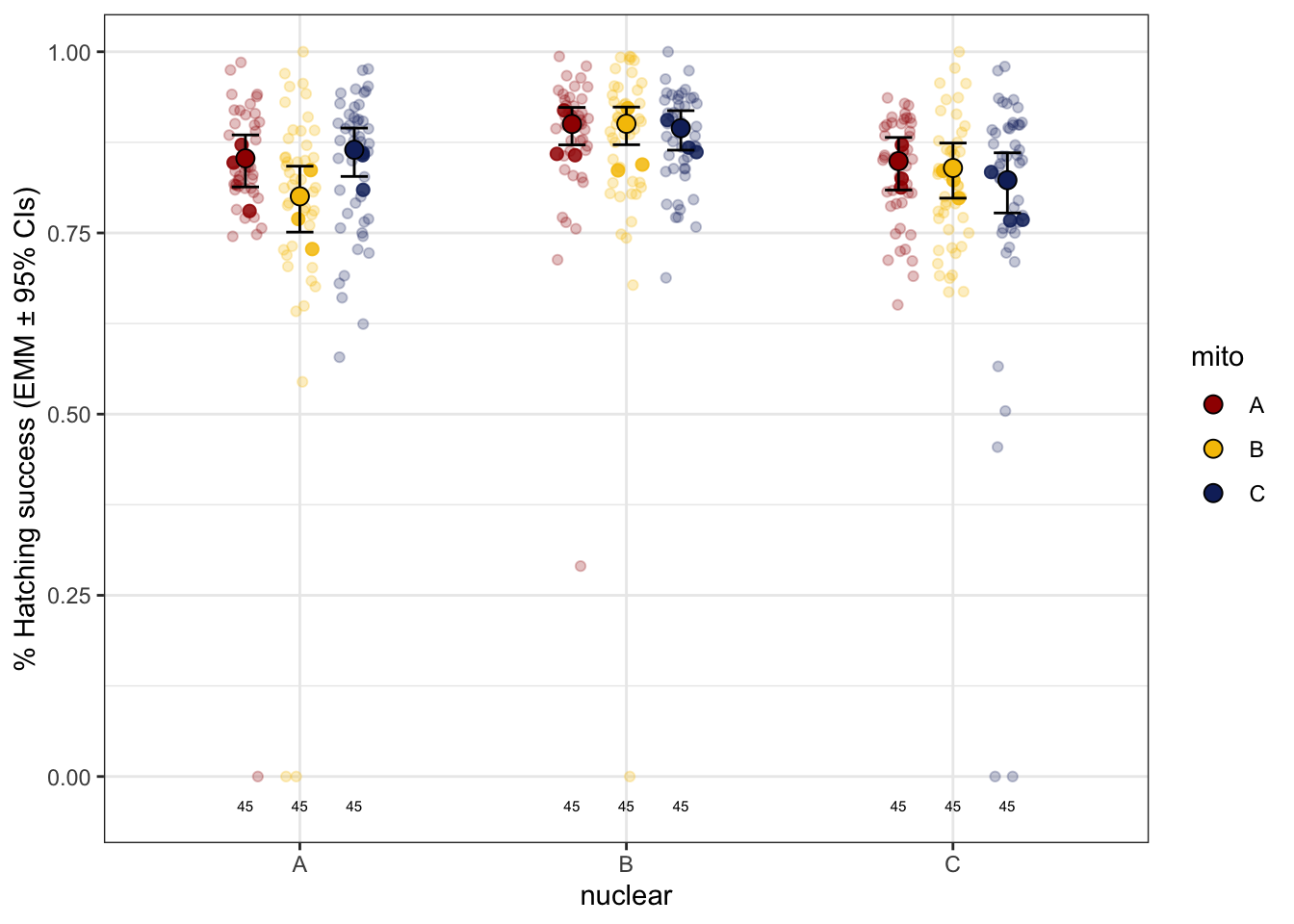

Past versions of unnamed-chunk-14-1.png

Version	Author	Date
a7bae31	MartinGarlovsky	2024-10-09

>>> Matched vs. mismatched

hatch_young_coevo <- glmer(cbind(total_offs, total_fail) ~ coevolved + (1|LINE) + (1|OLRE),
                           data = male_fert_filt %>% filter(age == "young"), 
                           family = 'binomial')

performance::check_model(hatch_young_coevo)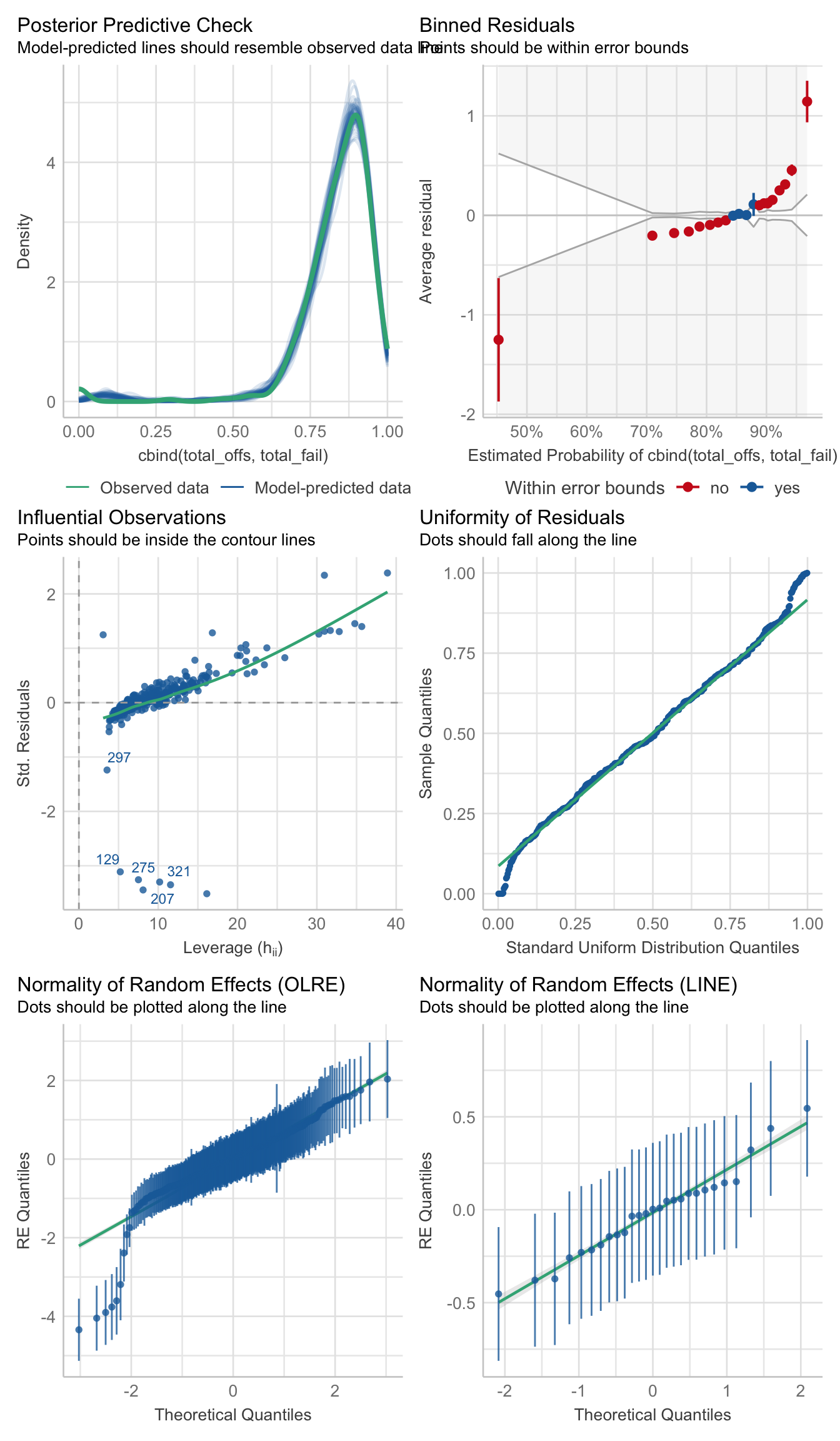

Past versions of unnamed-chunk-15-1.png

Version	Author	Date
0ffce9c	MartinGarlovsky	2024-10-10
a7bae31	MartinGarlovsky	2024-10-09

car::Anova(hatch_young_coevo, type = "3") %>% broom::tidy() %>% 
  as_tibble() %>% 
  kable(digits = 3, 
        caption = 'Analysis of Deviance Table (Type III Wald chisquare tests)') %>% 
  kable_styling(full_width = FALSE)

Analysis of Deviance Table (Type III Wald chisquare tests)

term	statistic	df	p.value
(Intercept)	565.895	1	0.000
coevolved	0.002	1	0.964

>>> Mito-type analysis

young_fert_snp <- glmer(cbind(total_offs, total_fail) ~ mito_snp * nuclear + (1|LINE) + (1|OLRE),
                        data = male_fert_filt %>% filter(age == "young"),
                        family = "binomial",
                        control = glmerControl(optimizer = "bobyqa", optCtrl = list(maxfun = 50000)))

performance::check_model(young_fert_snp)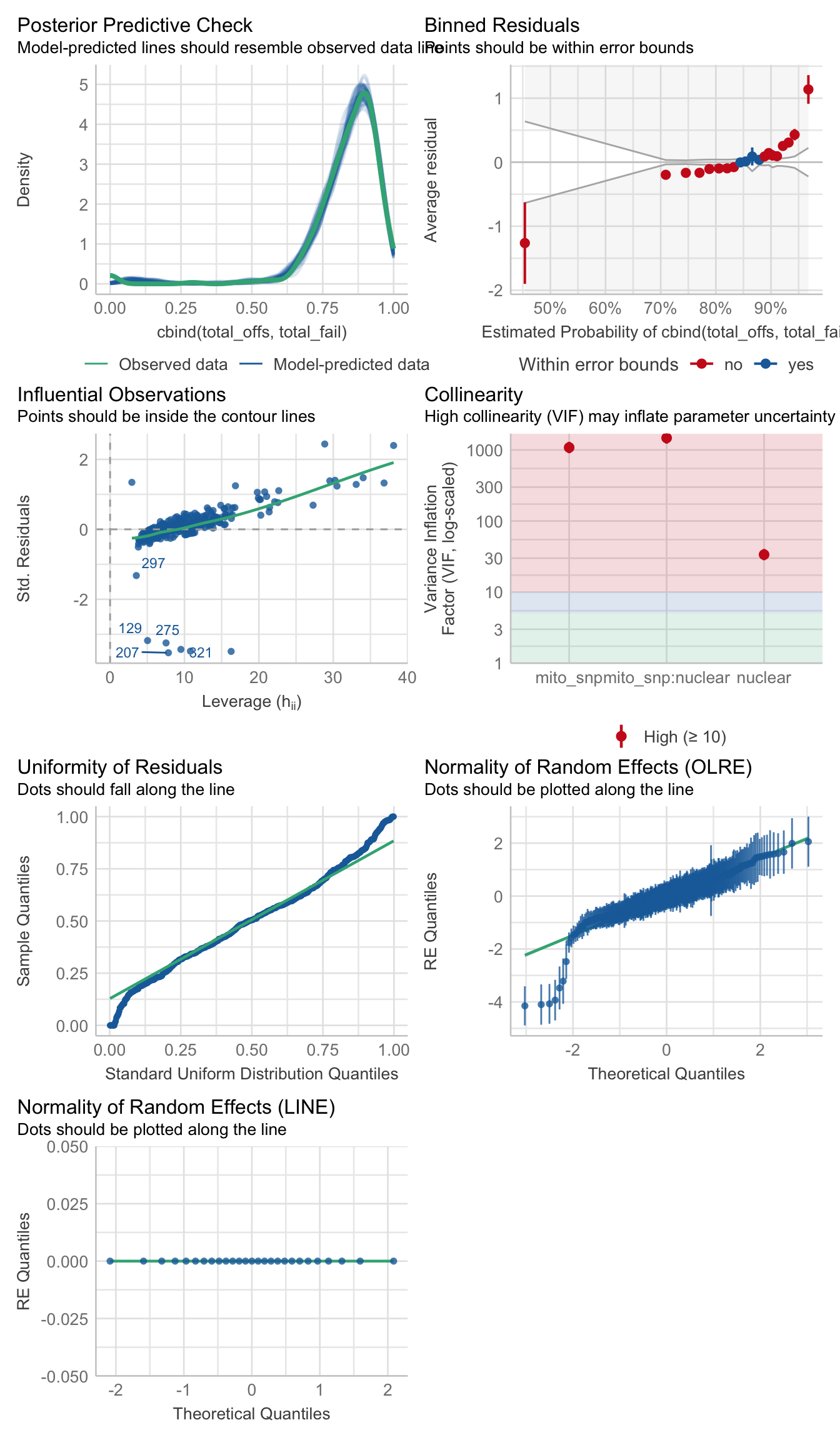

Past versions of unnamed-chunk-16-1.png

Version	Author	Date
0ffce9c	MartinGarlovsky	2024-10-10
a7bae31	MartinGarlovsky	2024-10-09

car::Anova(young_fert_snp, type = "3") %>% broom::tidy() %>% 
  as_tibble() %>% 
  kable(digits = 3, 
        caption = 'Analysis of Deviance Table (Type III Wald chisquare tests)') %>% 
  kable_styling(full_width = FALSE)

Analysis of Deviance Table (Type III Wald chisquare tests)

term	statistic	df	p.value
(Intercept)	118.245	1	0.000
mito_snp	10.256	8	0.248
nuclear	2.496	2	0.287
mito_snp:nuclear	9.013	7	0.252

>>> Old males

In old males we will model fertility as a binary variable - whether a male was fertile (1) or sterile (0). A stacked barchart of the binary response again clearly shows most young males are fertile, but a significant proporiton of old males fail to fertilise any eggs.

# add a new variable giving a binary fertile (1) or sterile (0) based on whether the proportion fertilised was 0 or greater than 0.
male_sterilty <- male_fert_filt %>% 
  mutate(sterility = if_else(fertilised == 0, 'sterile', 'fertile'),
         sterilbin = if_else(fertilised == 0, 0, 1),
         OLRE = 1:nrow(.))

male_sterilty %>% 
  group_by(mito, nuclear, age, sterility) %>% 
  count() %>% 
  ggplot(aes(x = nuclear, y = n, fill = sterility)) +
  geom_col(position = 'fill') + 
  labs(y = "Proportion of males") +
  facet_grid(mito ~ age)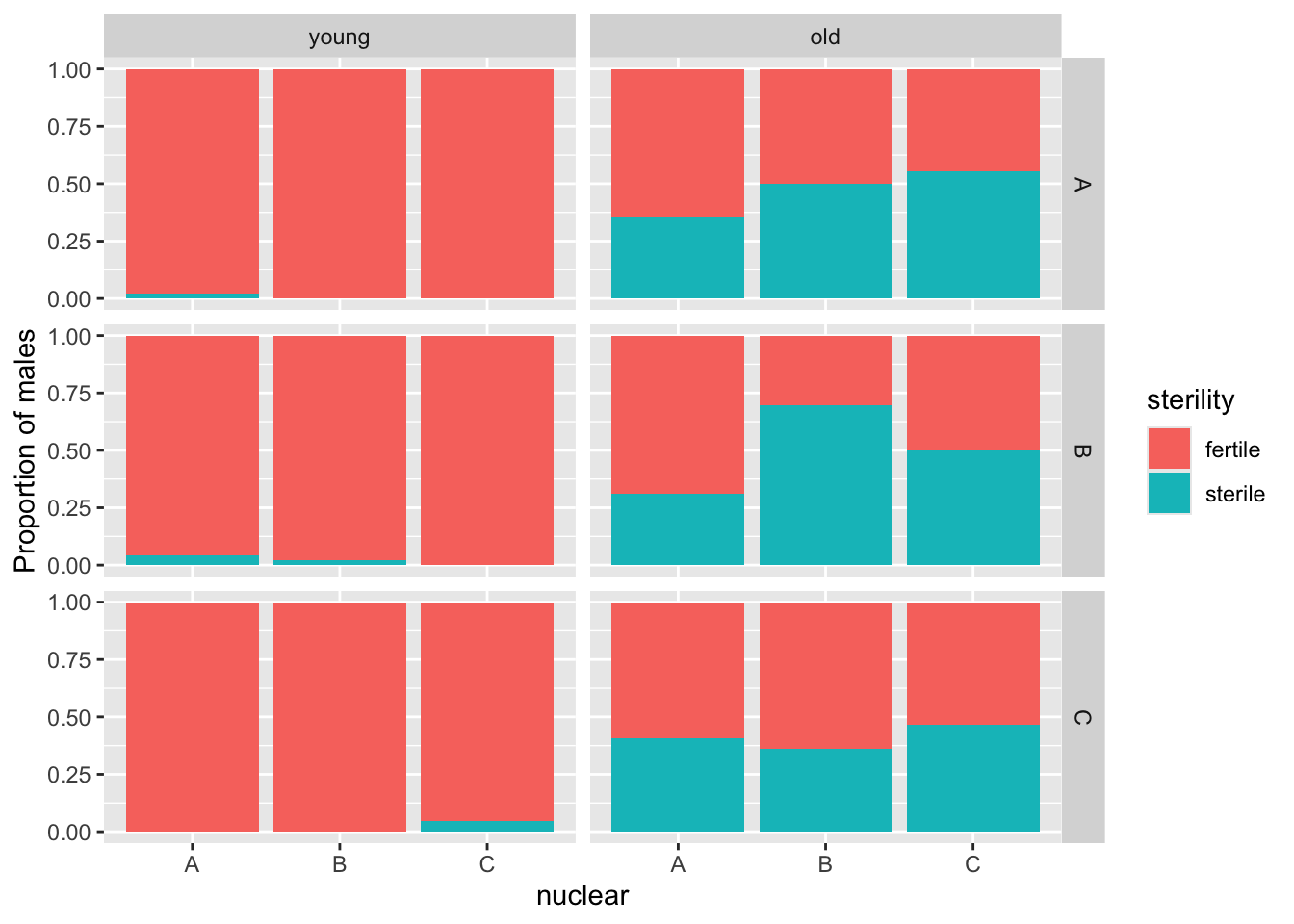

Past versions of unnamed-chunk-17-1.png

Version	Author	Date
a7bae31	MartinGarlovsky	2024-10-09

# model old males only
ster_md <- glmer(sterilbin ~ mito * nuclear + (1|LINE), family = 'binomial', 
                 data = male_sterilty %>% filter(age == "old"))

#summary(ster_md)

>>>> Check diagnostics

performance::check_model(ster_md)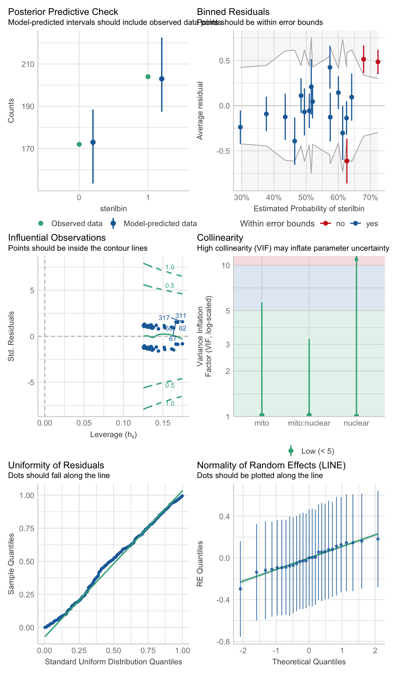

Past versions of unnamed-chunk-18-1.png

Version	Author	Date
0ffce9c	MartinGarlovsky	2024-10-10
a7bae31	MartinGarlovsky	2024-10-09

performance::check_overdispersion(ster_md)

# Overdispersion test

 dispersion ratio = 1.005
          p-value = 0.848

>>>> Results

car::Anova(ster_md, type = "3") %>% 
  broom::tidy() %>% 
  as_tibble() %>% #write_csv("output/anova_tables/male_fert_old.csv") %>% # save anova table for supp. tables
  kable(digits = 3, 
        caption = 'Analysis of Deviance Table (Type III Wald chisquare tests)') %>% 
  kable_styling(full_width = FALSE)

Analysis of Deviance Table (Type III Wald chisquare tests)

term	statistic	df	p.value
(Intercept)	1.819	1	0.177
mito	1.640	2	0.440
nuclear	6.819	2	0.033
mito:nuclear	6.935	4	0.139

ster_emm <- emmeans(ster_md, ~ mito * nuclear)

emmeans(ster_emm, pairwise ~ nuclear, adjust = "tukey")$contrasts %>% as_tibble() %>% 
  kable(digits = 3, 
        caption = 'Posthoc Tukey tests for comparison between nuclear genotypes') %>% 
  kable_styling(full_width = FALSE)

Posthoc Tukey tests for comparison between nuclear genotypes

contrast	estimate	SE	df	z.ratio	p.value
A - B	0.680	0.298	Inf	2.280	0.059
A - C	0.629	0.282	Inf	2.226	0.067
B - C	-0.051	0.294	Inf	-0.175	0.983

>>>>> Reaction norms

# reaction norms
hatchingsuccess_old_norm <- emmeans(ster_emm, ~ mito * nuclear, type = 'response') %>% as_tibble() %>% 
  ggplot(aes(x = nuclear, y = prob, fill = mito)) +
  geom_line(aes(group = mito, colour = mito), position = position_dodge(width = .5)) +
  geom_point(size = 3, pch = 21, position = position_dodge(width = .5)) +
  labs(y = 'Proportion fertile (EMM ± 95% CI)') +
  scale_colour_manual(values = met3) +
  scale_fill_manual(values = met3) +
  theme_bw() + 
  theme() +
  NULL

hatchingsuccess_old_norm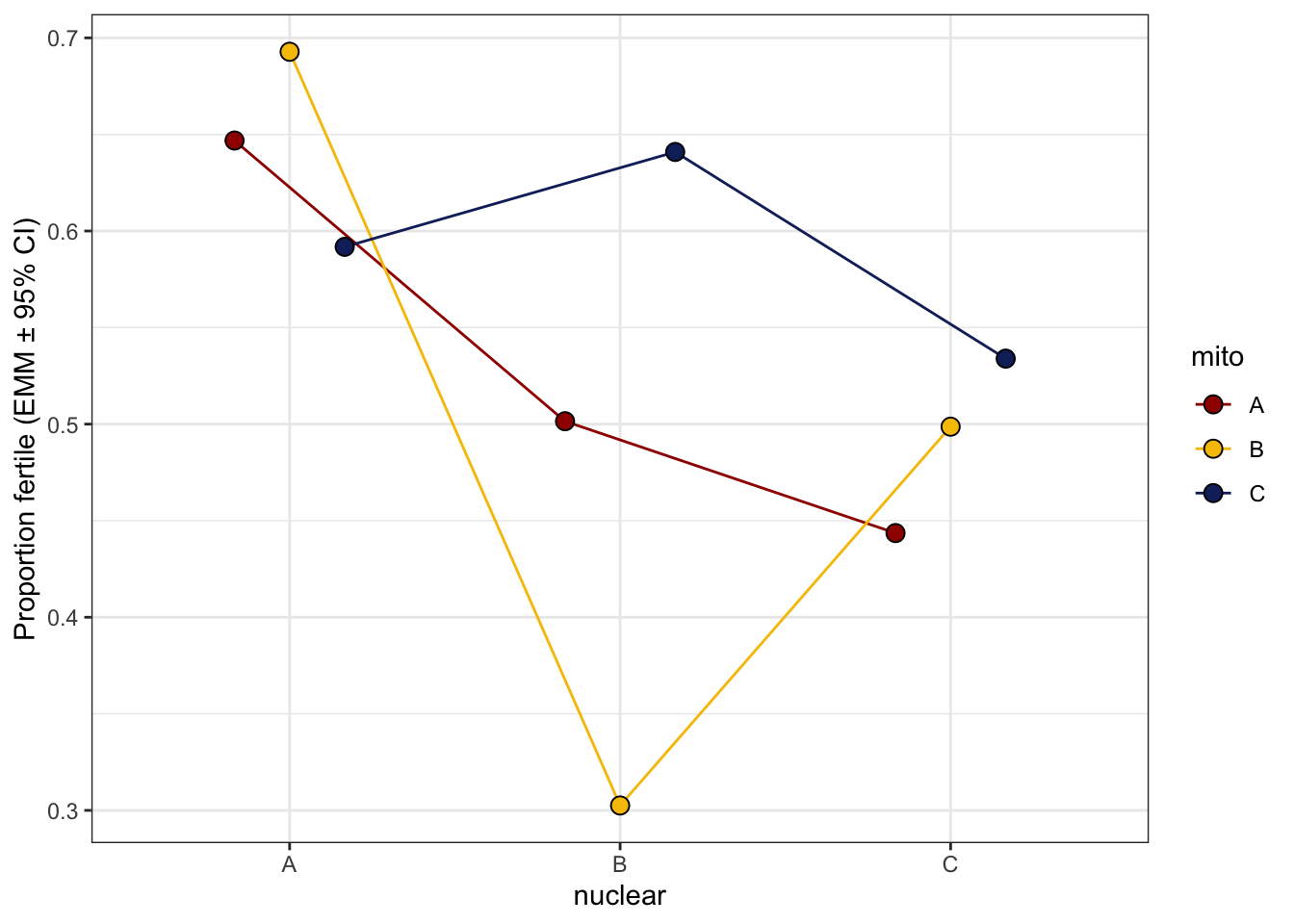

Past versions of unnamed-chunk-20-1.png

Version	Author	Date
a7bae31	MartinGarlovsky	2024-10-09

>>>>> Raw data and means

hatchingsuccess_old_raw <- emmeans(ster_emm, ~ mito * nuclear, type = 'response') %>% as_tibble() %>% 
  ggplot(aes(x = nuclear, y = prob, fill = mito)) +
  geom_jitter(data = male_fert_filt %>% filter(age == "old"),
              aes(y = fertilised, colour = mito),
               position = position_jitterdodge(dodge.width = .5, jitter.width = .1),
              alpha = .25) + 
  geom_jitter(data = male_fert_filt %>% filter(age == "old") %>% 
                group_by(LINE, age) %>% 
                summarise(mn = mean(fertilised)) %>% 
                separate(LINE, into = c("mito", "nuclear", NA), sep = "(?<=.)", remove = FALSE),
              aes(y = mn, colour = mito),
              position = position_jitterdodge(dodge.width = .5, jitter.width = .1),
              alpha = .85, size = 2) +
  geom_errorbar(aes(ymin = asymp.LCL, ymax = asymp.UCL), 
                width = .25, position = position_dodge(width = .5)) +
  geom_point(size = 3, pch = 21, position = position_dodge(width = .5)) +
  labs(y = 'Proportion fertile (EMM ± 95% CIs)') +
  scale_colour_manual(values = met3) +
  scale_fill_manual(values = met3) +
  theme_bw() + 
  theme() + 
  geom_text(data = male_fert_filt %>% filter(age == "young") %>% 
              group_by(mito, nuclear) %>% count(), aes(y = -0.04, label = n), 
            size = 2, position = position_dodge(width = .5)) + 
  #ggsave('figures/hatchingsuccess_old_raw.pdf', height = 4, width = 5, dpi = 600, useDingbats = FALSE) +
  NULL

hatchingsuccess_old_raw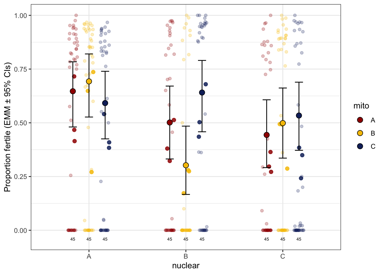

Past versions of unnamed-chunk-21-1.png

Version	Author	Date
a7bae31	MartinGarlovsky	2024-10-09

>>> Matched vs. mismatched

ster_coevo <- glmer(sterilbin ~ coevolved + (1|LINE), family = 'binomial', 
                    data = male_sterilty %>% filter(age == "old"))

car::Anova(ster_coevo, type = "3") %>% broom::tidy() %>% 
  as_tibble() %>% 
  kable(digits = 3, 
        caption = 'Analysis of Deviance Table (Type III Wald chisquare tests)') %>% 
  kable_styling(full_width = FALSE)

Analysis of Deviance Table (Type III Wald chisquare tests)

term	statistic	df	p.value
(Intercept)	0.749	1	0.387
coevolved	0.649	1	0.420

>>> Mito-type analysis

ster_md_snp <- glmer(sterilbin ~ mito_snp * nuclear + (1|LINE), 
                     family = 'binomial', 
                     data = male_sterilty %>% filter(age == "old"))

#summary(ster_md)

car::Anova(ster_md_snp, type = "3") %>% broom::tidy() %>% 
  as_tibble() %>% 
  kable(digits = 3, 
        caption = 'Analysis of Deviance Table (Type III Wald chisquare tests)') %>% 
  kable_styling(full_width = FALSE)

Analysis of Deviance Table (Type III Wald chisquare tests)

term	statistic	df	p.value
(Intercept)	1.084	1	0.298
mito_snp	5.792	8	0.671
nuclear	3.084	2	0.214
mito_snp:nuclear	9.564	7	0.215

>>>>> combined plot

comb_fert <- bind_rows(
  emmeans(hatch2, ~ mito * nuclear, type = 'response') %>% as_tibble() %>% mutate(age = "Young"),
  emmeans(ster_emm, ~ mito * nuclear, type = 'response') %>% as_tibble() %>% mutate(age = "Old")) %>% 
  mutate(age = fct_relevel(tolower(age), c("young", "old"))) %>% 
  ggplot(aes(x = nuclear, y = prob, fill = mito)) +
  geom_line(aes(group = mito, colour = mito), position = position_dodge(width = .5)) +
  # geom_errorbar(aes(ymin = asymp.LCL, ymax = asymp.UCL), 
  #               width = .25, position = position_dodge(width = .5)) +
  geom_point(size = 3, pch = 21, position = position_dodge(width = .5)) +
  labs(y = 'Proportion fertile (EMM ± 95% CI)') +
  scale_colour_manual(values = met3) +
  scale_fill_manual(values = met3) +
  facet_wrap(~age) +
  theme_bw() + 
  theme() +
  NULL

comb_fert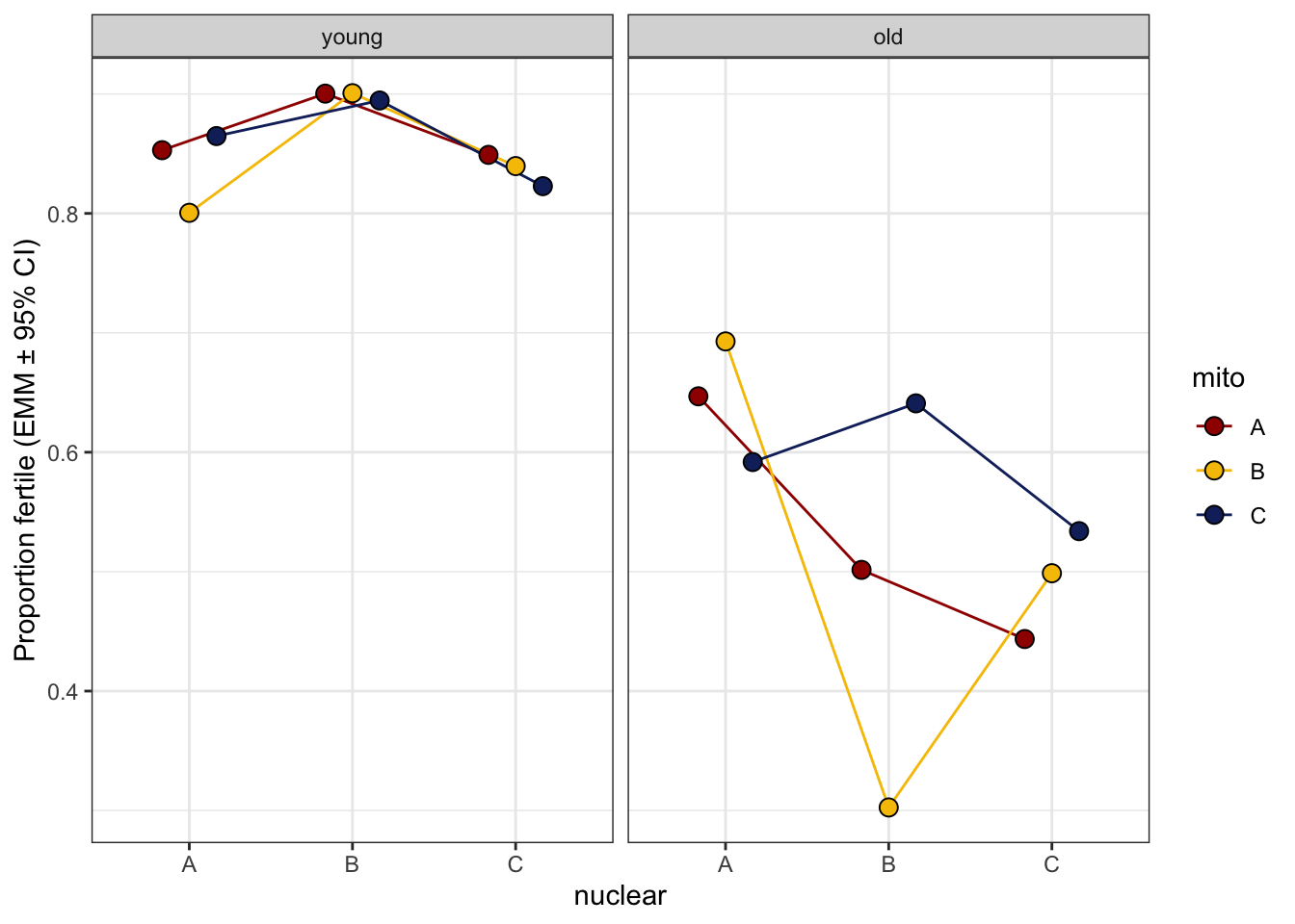

Past versions of unnamed-chunk-24-1.png

Version	Author	Date
a7bae31	MartinGarlovsky	2024-10-09

> Sperm viability

We measured sperm viability using live/dead staining in a control medium (t0 = c) and after 30mins in a stressor medium (t30 = t). First, we analysed control and treatment separately. For the measurement of sperm viability, we collected all males on a single day for each block. However, the dissection, staining and incubation protocol necessitated measurements were carried out over several days. The measurement of sperm viability in young males (collected at 5 days old) thus extended for 8 days and that of old males (collected at 6 weeks old) for 6 days. To account for this variation in age we included dissection day (an extension of male age) and block as fixed covariates.

The sperm viability models returned a singularity warning message due to a zero-variance component estimate for the line random effect intercept. We retained these models after trying a range of alternatives and checking simplified models without the random slopes term that all resulted in the same qualitative findings for the fixed effects part of the model.

sperm_vib_filt %>% 
  group_by(mito, nuclear, age, treatment) %>% 
  summarise(mn = mean(viability),
            se = sd(viability)/sqrt(n()),
            s95 = se * 1.96) %>% 
  ggplot(aes(x = nuclear, y = mn, fill = mito)) +
  geom_point(data = sperm_vib_filt %>% 
               group_by(mito, nuclear, age, treatment, male_ID) %>% 
               summarise(viability = mean(viability)),
             aes(y = viability, colour = mito), alpha = .15,
             position = position_jitterdodge(dodge.width = .5, jitter.width = .1)) +
  geom_errorbar(aes(ymin = mn - s95, ymax = mn + s95), 
                width = .25, position = position_dodge(width = .5)) +
  geom_line(aes(group = mito), position = position_dodge(width = .5)) + 
  geom_point(size = 3, pch = 21, position = position_dodge(width = .5)) +
  labs(y = 'Sperm viability') +
  facet_grid(treatment ~ age, scales = 'free_x') +
  scale_colour_manual(values = met3) +
  scale_fill_manual(values = met3) +
  theme_bw() + 
  theme() + 
  NULL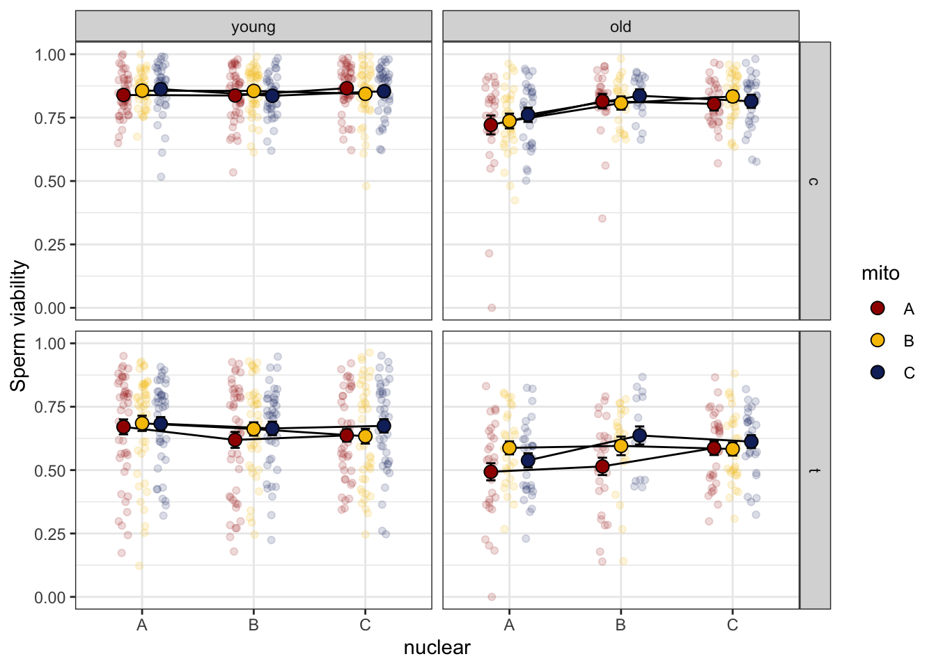

Past versions of unnamed-chunk-25-1.png

Version	Author	Date
a7bae31	MartinGarlovsky	2024-10-09

>>> Control treatment (t0)

First we take a look at the data to see how response changes with the covariates.

>>>> Day effect

spvfilt_control <- sperm_vib_filt %>% filter(treatment == 'c')

spvfilt_control %>% 
  group_by(mito, nuclear, age, days) %>% 
  summarise(mn = mean(viability),
            se = sd(viability)/sqrt(n()),
            s95 = se * 1.96) %>% 
  ggplot(aes(x = nuclear, y = mn, fill = mito)) +
  geom_point(data = spvfilt_control %>% 
                group_by(mito, nuclear, age, days, male_ID) %>% summarise(viability = mean(viability)),
             aes(y = viability, colour = mito), alpha = .15,
             position = position_jitterdodge(dodge.width = .5, jitter.width = .1)) +
  geom_errorbar(aes(ymin = mn - s95, ymax = mn + s95), 
                width = .25, position = position_dodge(width = .5)) +
  geom_line(aes(group = mito, colour = mito), position = position_dodge(width = .5)) + 
  geom_point(size = 3, pch = 21, position = position_dodge(width = .5)) +
  labs(y = 'Sperm viability') +
  facet_grid(age ~ days, scales = 'free_x') +
  scale_colour_manual(values = met3) +
  scale_fill_manual(values = met3) +
  theme_bw() + 
  theme() + 
  NULL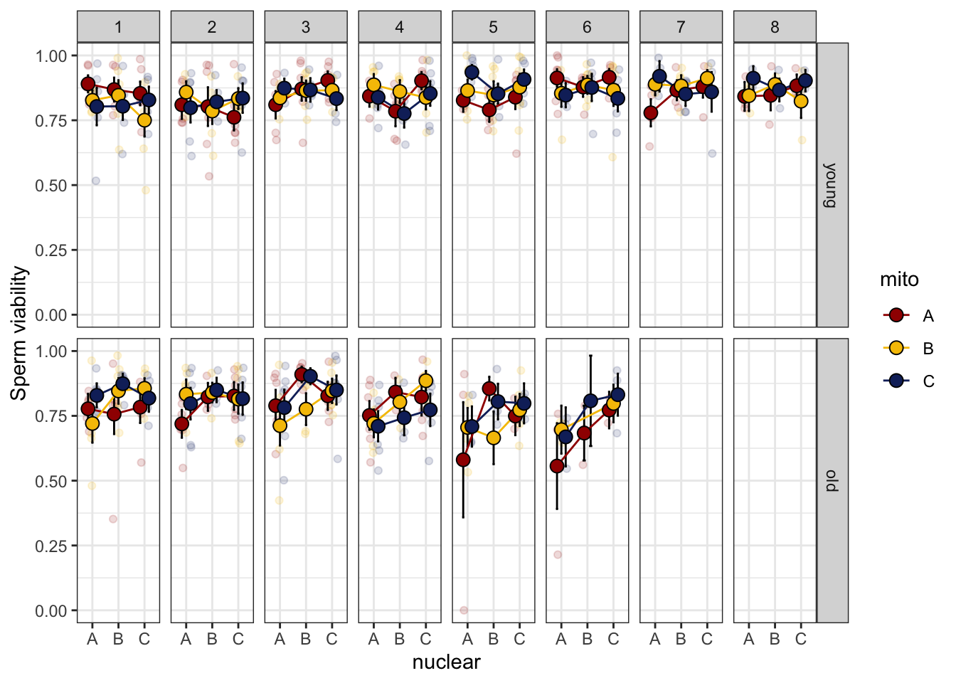

Past versions of unnamed-chunk-26-1.png

Version	Author	Date
a7bae31	MartinGarlovsky	2024-10-09

>>>> Block effect

spvfilt_control %>% 
  group_by(mito, nuclear, age, block) %>% 
  summarise(mn = mean(viability),
            se = sd(viability)/sqrt(n()),
            s95 = se * 1.96) %>% 
  ggplot(aes(x = nuclear, y = mn, fill = mito)) +
  geom_point(data = spvfilt_control %>% 
                group_by(mito, nuclear, age, block, male_ID) %>% summarise(viability = mean(viability)),
             aes(y = viability, colour = mito), alpha = .15,
             position = position_jitterdodge(dodge.width = .5, jitter.width = .1)) +
  geom_errorbar(aes(ymin = mn - s95, ymax = mn + s95), 
                width = .25, position = position_dodge(width = .5)) +
  geom_line(aes(group = mito, colour = mito), position = position_dodge(width = .5)) + 
  geom_point(size = 3, pch = 21, position = position_dodge(width = .5)) +
  labs(y = 'Sperm viability') +
  facet_grid(age ~ block, scales = 'free_x') +
  scale_colour_manual(values = met3) +
  scale_fill_manual(values = met3) +
  theme_bw() + 
  theme() + 
  NULL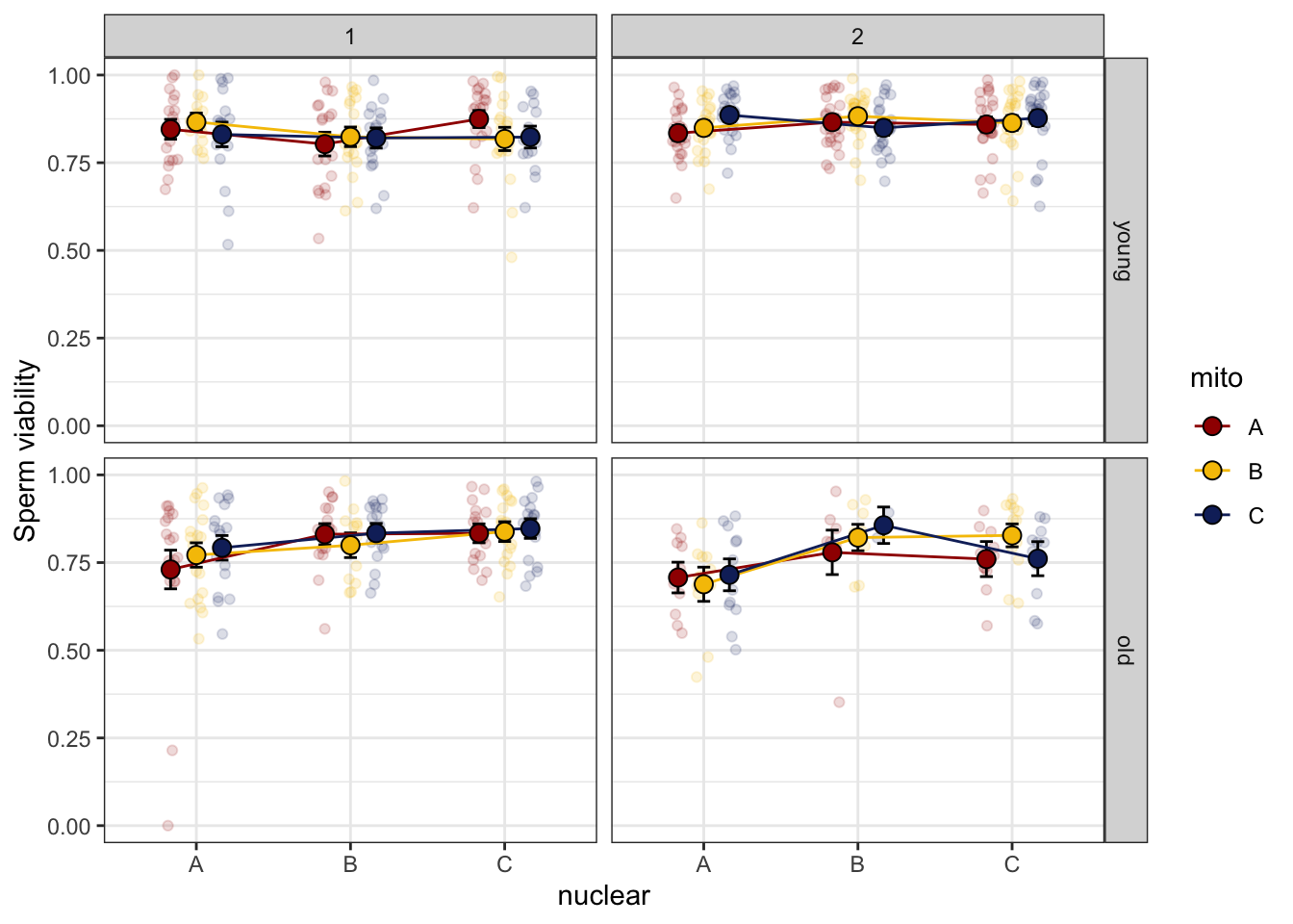

Past versions of unnamed-chunk-27-1.png

Version	Author	Date
a7bae31	MartinGarlovsky	2024-10-09

>>> Results

viability_m1 <- glmer(cbind(live, dead) ~ mito * nuclear * age + days + block + (1|LINE:age) + (1|male_ID) + (1|OLRE),
                      data = spvfilt_control, family = 'binomial',
                   control = glmerControl(optimizer = "bobyqa", optCtrl = list(maxfun = 50000)))

>>>> Check diagnostics

performance::check_model(viability_m1)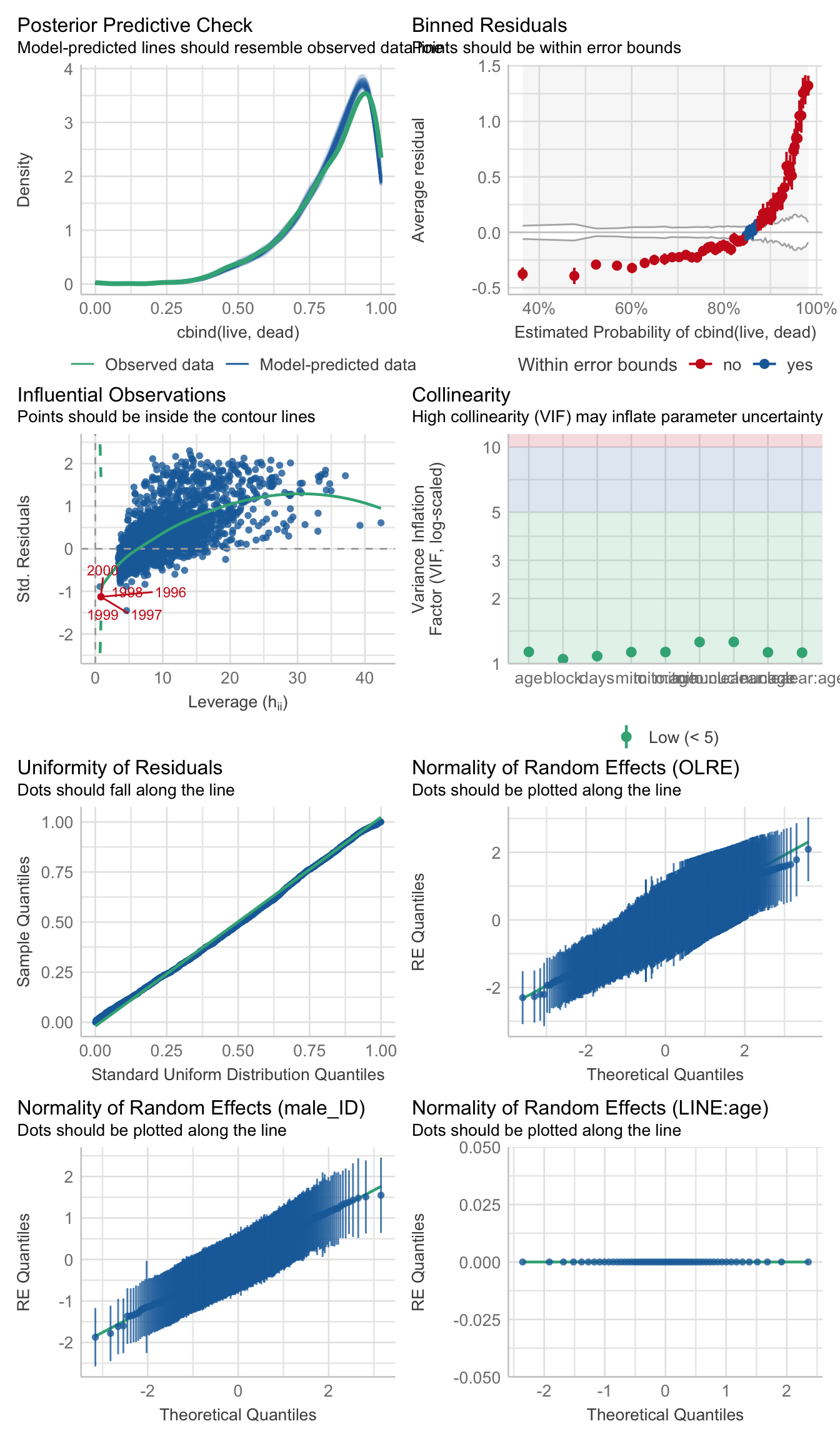

Past versions of unnamed-chunk-29-1.png

Version	Author	Date
0ffce9c	MartinGarlovsky	2024-10-10
a7bae31	MartinGarlovsky	2024-10-09

performance::check_overdispersion(viability_m1)

# Overdispersion test

 dispersion ratio =   0.625
          p-value = < 0.001

# diagnostics
testDispersion(viability_m1)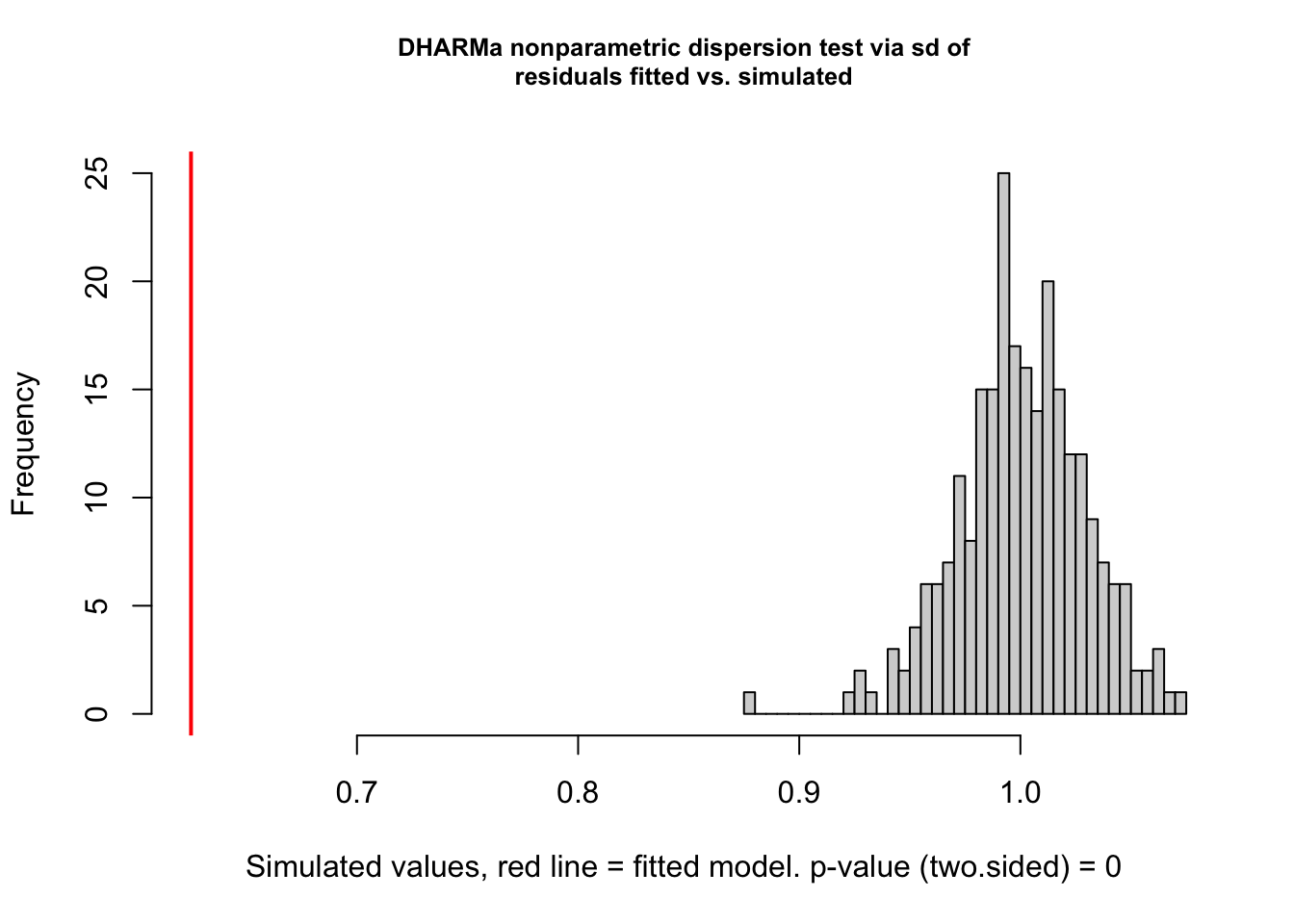

Past versions of unnamed-chunk-30-1.png

Version	Author	Date
a7bae31	MartinGarlovsky	2024-10-09

    DHARMa nonparametric dispersion test via sd of residuals fitted vs.
    simulated

data:  simulationOutput
dispersion = 0.62462, p-value < 2.2e-16
alternative hypothesis: two.sided

simulationOutput <- simulateResiduals(fittedModel = viability_m1, plot = FALSE)
hist(residuals(simulationOutput))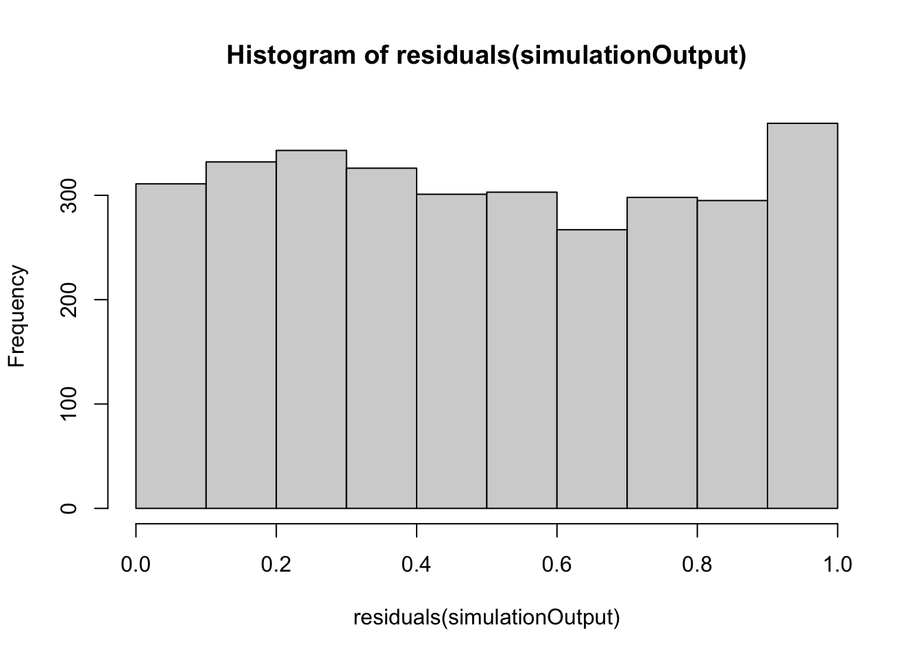

Past versions of unnamed-chunk-30-2.png

Version	Author	Date
a7bae31	MartinGarlovsky	2024-10-09

hist(residuals(simulationOutput, quantileFunction = qnorm, outlierValues = c(-7,7)))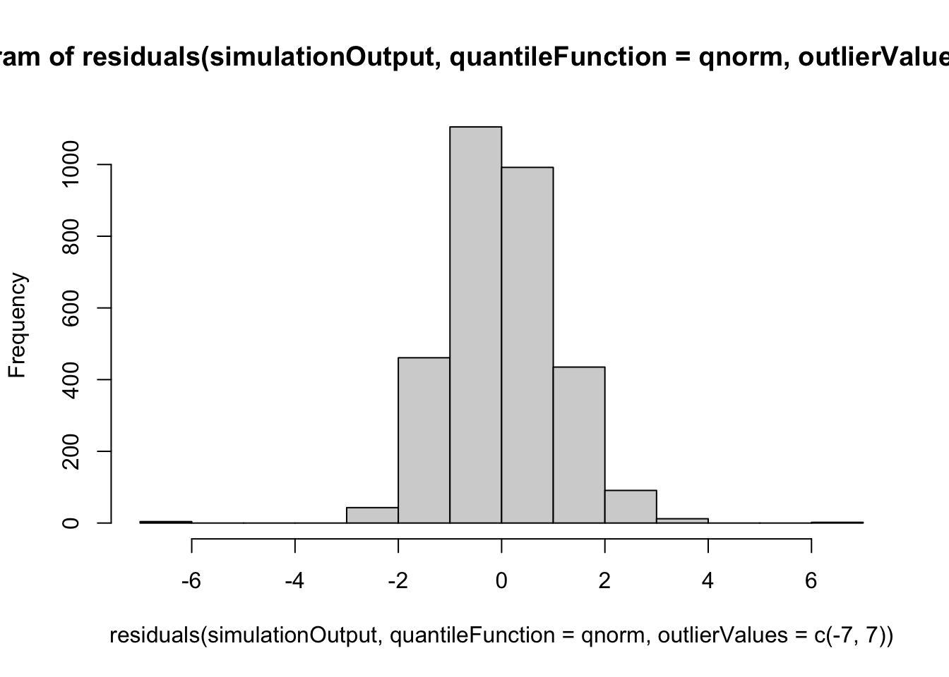

Past versions of unnamed-chunk-30-3.png

Version	Author	Date
a7bae31	MartinGarlovsky	2024-10-09

plot(simulationOutput)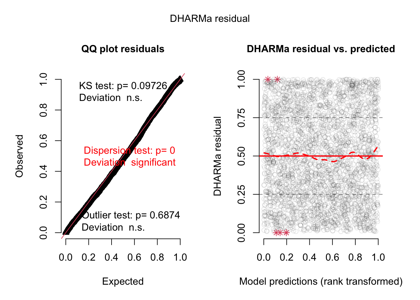

Past versions of unnamed-chunk-30-4.png

Version	Author	Date
a7bae31	MartinGarlovsky	2024-10-09

>>>>

car::Anova(viability_m1, type = "3") %>% 
  broom::tidy() %>% 
  #write_csv("output/anova_tables/viability_t0.csv") %>% # save anova table for supp. tables
  as_tibble() %>% 
  kable(digits = 3, 
        caption = 'Analysis of Deviance Table (Type III Wald chisquare tests)') %>% 
  kable_styling(full_width = FALSE)

Analysis of Deviance Table (Type III Wald chisquare tests)

term	statistic	df	p.value
(Intercept)	241.616	1	0.000
mito	0.986	2	0.611
nuclear	13.078	2	0.001
age	34.305	1	0.000
days	2.467	1	0.116
block	0.389	1	0.533
mito:nuclear	1.755	4	0.781
mito:age	0.125	2	0.939
nuclear:age	13.100	2	0.001
mito:nuclear:age	3.910	4	0.418

#summary(viability_m1)

# posthoc tests
bind_rows(emmeans(viability_m1, pairwise ~ age | nuclear, adjust = "tukey")$contrasts %>% broom::tidy(),
          emmeans(viability_m1, pairwise ~ nuclear | age, adjust = "tukey")$contrasts %>% broom::tidy() %>%
            rename(p.value = adj.p.value)) %>% 
  mutate(p.val = ifelse(p.value < 0.001, '< 0.001', round(p.value, 3))) %>% 
  select(-p.value, -term) %>% relocate(age, .before = contrast) %>% 
  kable(digits = 3, 
        caption = 'Posthoc Tukey tests to compare which groups differ') %>% 
  kable_styling(full_width = FALSE) %>%
  kableExtra::group_rows("Age", 1, 3) %>%
  kableExtra::group_rows("Nuclear - old", 4, 6) %>%
  kableExtra::group_rows("Nuclear - young", 7, 9)

Posthoc Tukey tests to compare which groups differ

nuclear	age	contrast	null.value	estimate	std.error	df	statistic	p.val
Age
A	NA	young - old	0	0.750	0.114	Inf	6.574	< 0.001
B	NA	young - old	0	0.179	0.128	Inf	1.397	0.163
C	NA	young - old	0	0.319	0.114	Inf	2.797	0.005
Nuclear - old
NA	young	A - B	0	0.095	0.104	Inf	0.919	0.628
NA	young	A - C	0	-0.067	0.104	Inf	-0.647	0.794
NA	young	B - C	0	-0.162	0.103	Inf	-1.574	0.257
Nuclear - young
NA	old	A - B	0	-0.476	0.133	Inf	-3.582	< 0.001
NA	old	A - C	0	-0.499	0.121	Inf	-4.134	< 0.001
NA	old	B - C	0	-0.023	0.133	Inf	-0.170	0.984

>>>> Reaction norms

sperm_vib_norm <- emmeans(viability_m1, ~ mito * nuclear * age, type = 'response') %>% as_tibble() %>% 
  ggplot(aes(x = nuclear, y = prob, fill = mito)) +
  geom_line(aes(group = mito, colour = mito), position = position_dodge(width = .5)) +
  # geom_errorbar(aes(ymin = asymp.LCL, ymax = asymp.UCL),
  #               width = .25, position = position_dodge(width = .5)) +
  geom_point(size = 3, pch = 21, position = position_dodge(width = .5)) +
  labs(y = 'Sperm viability (EMM)') +
  scale_colour_manual(values = met3) +
  scale_fill_manual(values = met3) +
  #scale_y_continuous(limits = c(0, 1.05)) +
  facet_wrap(~ age) +
  theme_bw() + 
  theme() + 
  NULL

sperm_vib_norm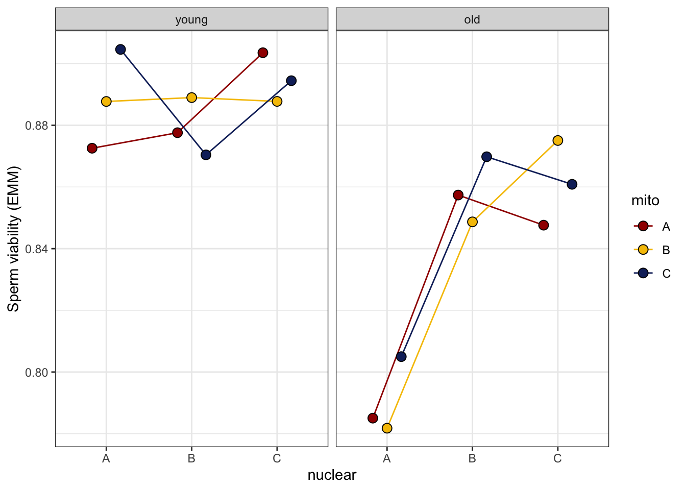

Past versions of unnamed-chunk-32-1.png

Version	Author	Date
a7bae31	MartinGarlovsky	2024-10-09

>>>> Raw data and means

sperm_vib_raw <- emmeans(viability_m1, ~ mito * nuclear * age, type = 'response') %>% as_tibble() %>% 
  ggplot(aes(x = nuclear, y = prob, fill = mito)) +
  geom_jitter(data = spvfilt_control %>% 
               group_by(mito, nuclear, age, treatment, male_ID) %>% 
               summarise(viability = mean(viability)),
              aes(y = viability, colour = mito),
               position = position_jitterdodge(dodge.width = .5, jitter.width = .1),
              size = 0.75, alpha = .1) +
  geom_jitter(data = spvfilt_control %>% 
                group_by(LINE, age) %>% 
                summarise(mn = mean(viability)) %>% 
                separate(LINE, into = c("mito", "nuclear", NA), sep = "(?<=.)", remove = FALSE),
              aes(y = mn, colour = mito),
              position = position_jitterdodge(dodge.width = .5, jitter.width = .1),
              alpha = .85, size = 2) +
  geom_errorbar(aes(ymin = asymp.LCL, ymax = asymp.UCL), 
                width = .25, position = position_dodge(width = .5)) +
  geom_point(size = 3, pch = 21, position = position_dodge(width = .5)) +
  labs(y = 'Sperm viability (EMM ± 95% CIs)') +
  scale_colour_manual(values = met3) +
  scale_fill_manual(values = met3) +
  facet_wrap(~ age) +
  theme_bw() + 
  theme() + 
  geom_text(data = spvfilt_control %>% 
              group_by(mito, nuclear, age) %>% 
              summarise(N = n_distinct(male_ID)), 
            aes(y = -0.04, label = N), 
            size = 2, position = position_dodge(width = .5)) + 
  #ggsave('figures/sperm_vib_contrl_supp.pdf', height = 4, width = 8, dpi = 600, useDingbats = FALSE) +
  NULL

sperm_vib_raw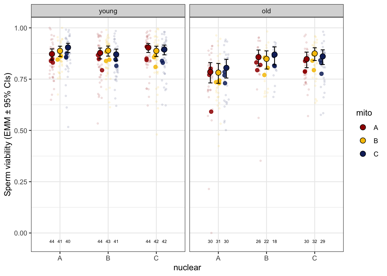

Past versions of unnamed-chunk-33-1.png

Version	Author	Date
a7bae31	MartinGarlovsky	2024-10-09

Matched vs. mismatched

viability_coevo <- glmer(cbind(live, dead) ~ coevolved * age + days + block + (age|LINE) + (1|male_ID) + (1|OLRE),
                      data = spvfilt_control, family = 'binomial')

car::Anova(viability_coevo, type = "3")

Analysis of Deviance Table (Type III Wald chisquare tests)

Response: cbind(live, dead)
                 Chisq Df Pr(>Chisq)    
(Intercept)   222.9440  1  < 2.2e-16 ***
coevolved       0.2777  1     0.5982    
age            28.5398  1  9.179e-08 ***
days            2.3157  1     0.1281    
block           0.4828  1     0.4872    
coevolved:age   0.0162  1     0.8988    
---
Signif. codes:  0 '***' 0.001 '**' 0.01 '*' 0.05 '.' 0.1 ' ' 1

Mito-type analysis

viability_snp <- glmer(cbind(live, dead) ~ mito_snp * nuclear * age + 
                         days + block + (1 + age|LINE) + (1|male_ID) + (1|OLRE),
                       data = spvfilt_control, family = 'binomial',
                       control= glmerControl(optimizer="bobyqa", optCtrl=list(maxfun=50000)))

car::Anova(viability_snp, type = "3")

Analysis of Deviance Table (Type III Wald chisquare tests)

Response: cbind(live, dead)
                       Chisq Df Pr(>Chisq)    
(Intercept)          94.0598  1  < 2.2e-16 ***
mito_snp              6.2862  8   0.615205    
nuclear               0.2596  2   0.878279    
age                   6.9185  1   0.008531 ** 
days                  2.5477  1   0.110455    
block                 0.4244  1   0.514727    
mito_snp:nuclear      6.5456  7   0.477669    
mito_snp:age          3.1756  8   0.922859    
nuclear:age           4.1995  2   0.122486    
mito_snp:nuclear:age  5.3770  7   0.614063    
---
Signif. codes:  0 '***' 0.001 '**' 0.01 '*' 0.05 '.' 0.1 ' ' 1

>> Stress treatment (t30)

spvfilt_treat <- sperm_vib_filt %>% filter(treatment == 't')

>>>> Day effect

spvfilt_treat %>% 
  group_by(mito, nuclear, age, block) %>% 
  summarise(mn = mean(viability),
            se = sd(viability)/sqrt(n()),
            s95 = se * 1.96) %>% 
  ggplot(aes(x = nuclear, y = mn, fill = mito)) +
  geom_point(data = spvfilt_treat %>% 
                group_by(mito, nuclear, age, block, male_ID) %>% summarise(viability = mean(viability)),
             aes(y = viability, colour = mito), alpha = .15,
             position = position_jitterdodge(dodge.width = .5, jitter.width = .1)) +
  geom_errorbar(aes(ymin = mn - s95, ymax = mn + s95), 
                width = .25, position = position_dodge(width = .5)) +
  geom_line(aes(group = mito), position = position_dodge(width = .5)) + 
  geom_point(size = 3, pch = 21, position = position_dodge(width = .5)) +
  labs(y = 'Sperm viability') +
  facet_grid(age ~ block, scales = 'free_x') +
  scale_colour_manual(values = met3) +
  scale_fill_manual(values = met3) +
  theme_bw() + 
  theme() + 
  NULL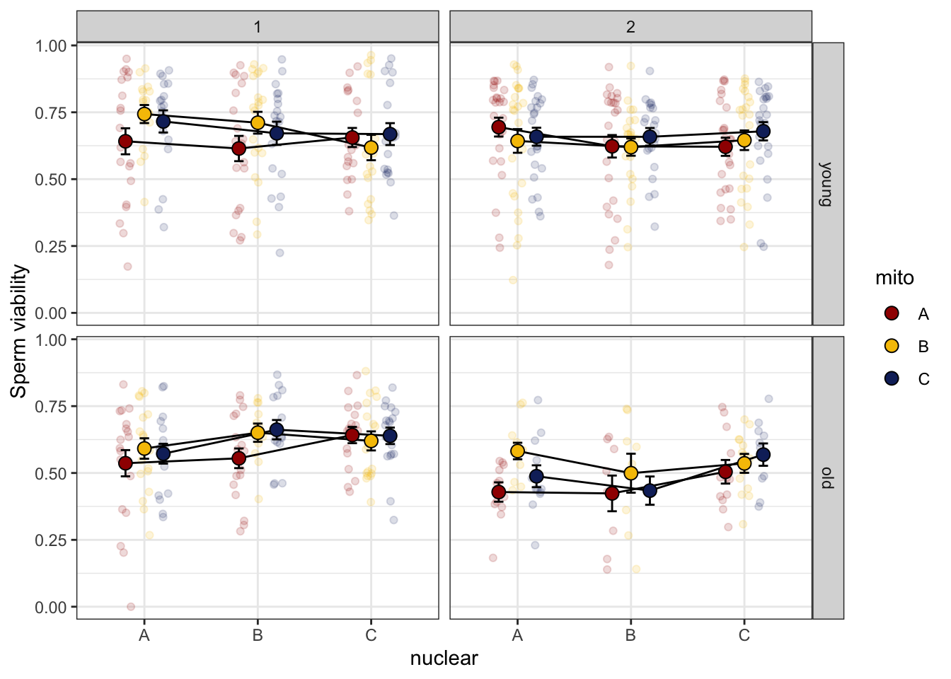

Past versions of unnamed-chunk-37-1.png

Version	Author	Date
a7bae31	MartinGarlovsky	2024-10-09

>>>> Block effect

spvfilt_treat %>% 
  group_by(mito, nuclear, age, days) %>% 
  summarise(mn = mean(viability),
            se = sd(viability)/sqrt(n()),
            s95 = se * 1.96) %>% 
  ggplot(aes(x = nuclear, y = mn, fill = mito)) +
  geom_point(data = spvfilt_treat %>% 
                group_by(mito, nuclear, age, days, male_ID) %>% summarise(viability = mean(viability)),
             aes(y = viability, colour = mito), alpha = .15,
             position = position_jitterdodge(dodge.width = .5, jitter.width = .1)) +
  geom_errorbar(aes(ymin = mn - s95, ymax = mn + s95), 
                width = .25, position = position_dodge(width = .5)) +
  geom_line(aes(group = mito), position = position_dodge(width = .5)) + 
  geom_point(size = 3, pch = 21, position = position_dodge(width = .5)) +
  labs(y = 'Sperm viability') +
  facet_grid(age ~ days, scales = 'free_x') +
  scale_colour_manual(values = met3) +
  scale_fill_manual(values = met3) +
  theme_bw() + 
  theme() + 
  NULL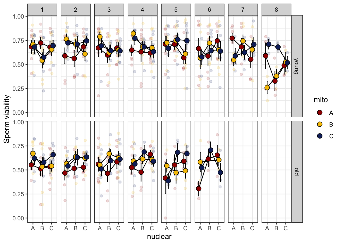

Past versions of unnamed-chunk-38-1.png

Version	Author	Date
a7bae31	MartinGarlovsky	2024-10-09

>>> Results

# model
viability_m2 <- glmer(cbind(live, dead) ~ mito * nuclear * age + days + block + (1 + age|LINE) + (1|male_ID) + (1|OLRE),
                      data = spvfilt_treat, family = 'binomial',
                      control = glmerControl(optimizer = "bobyqa", optCtrl = list(maxfun = 50000)))

>>>> Check diagnostics

performance::check_model(viability_m2)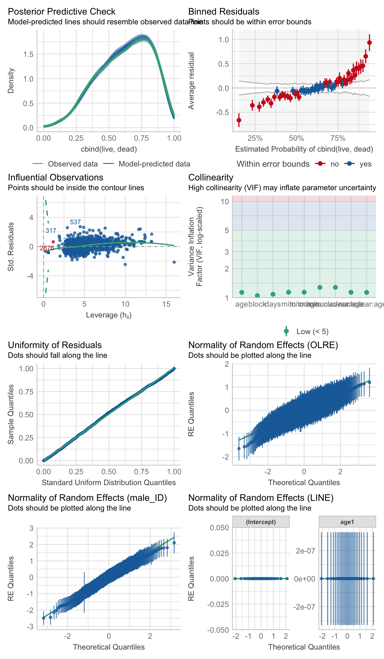

Past versions of unnamed-chunk-40-1.png

Version	Author	Date
0ffce9c	MartinGarlovsky	2024-10-10
a7bae31	MartinGarlovsky	2024-10-09

performance::check_overdispersion(viability_m2)

# Overdispersion test

 dispersion ratio =   0.854
          p-value = < 0.001

testDispersion(viability_m2)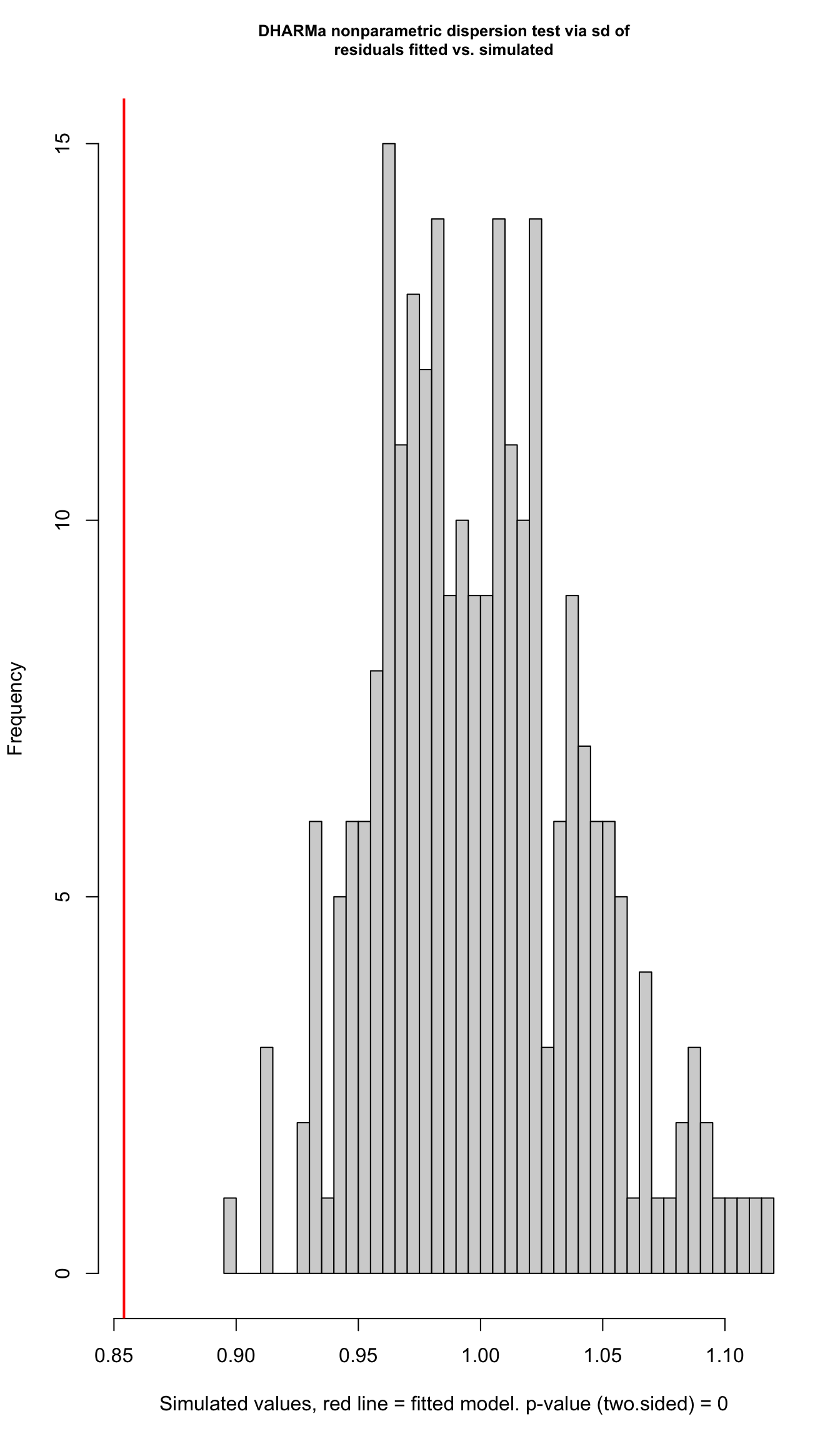

Past versions of unnamed-chunk-41-1.png

Version	Author	Date
a7bae31	MartinGarlovsky	2024-10-09

    DHARMa nonparametric dispersion test via sd of residuals fitted vs.
    simulated

data:  simulationOutput
dispersion = 0.85413, p-value < 2.2e-16
alternative hypothesis: two.sided

simulationOutput <- simulateResiduals(fittedModel = viability_m2, plot = FALSE)
hist(residuals(simulationOutput))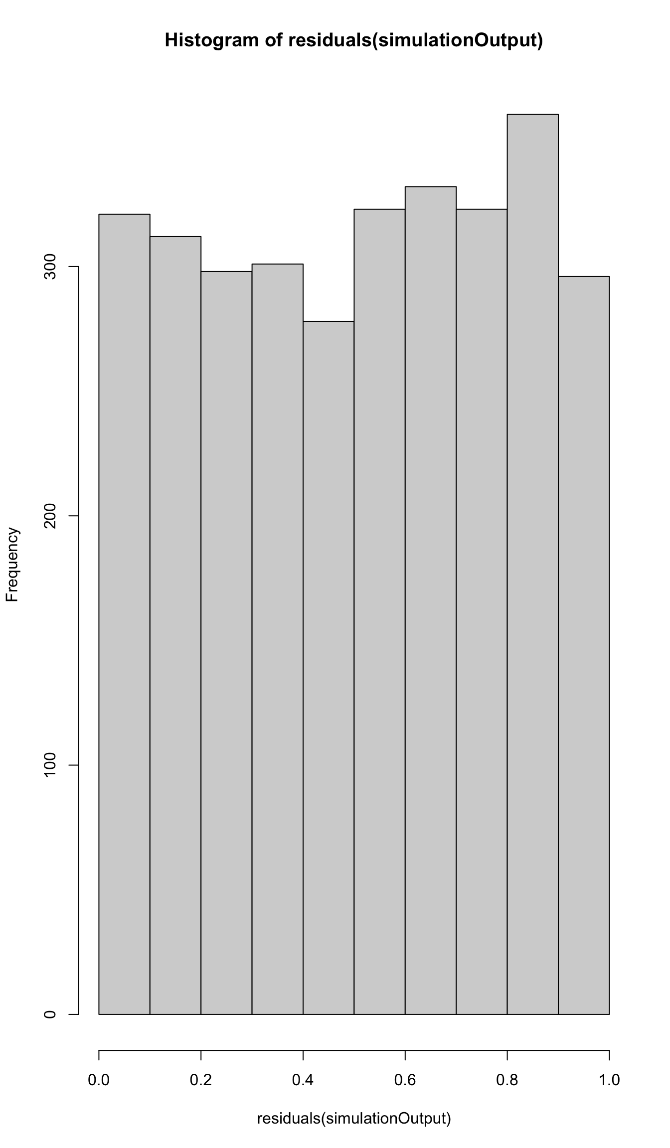

Past versions of unnamed-chunk-41-2.png

Version	Author	Date
a7bae31	MartinGarlovsky	2024-10-09

hist(residuals(simulationOutput, quantileFunction = qnorm, outlierValues = c(-7,7)))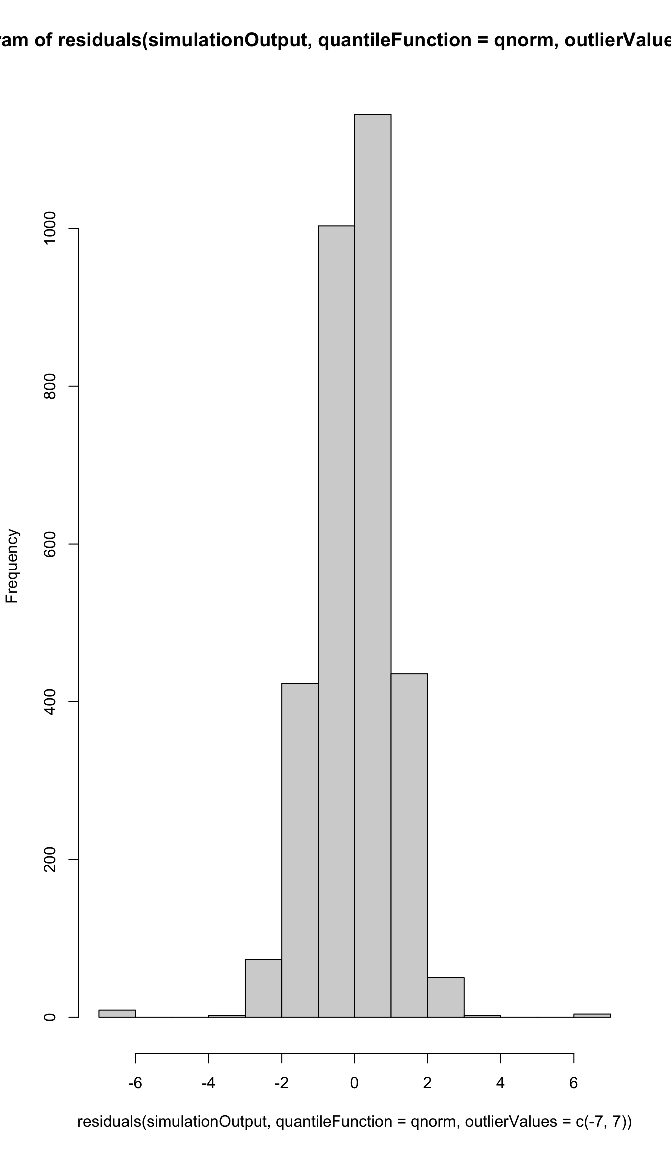

Past versions of unnamed-chunk-41-3.png

Version	Author	Date
a7bae31	MartinGarlovsky	2024-10-09

plot(simulationOutput)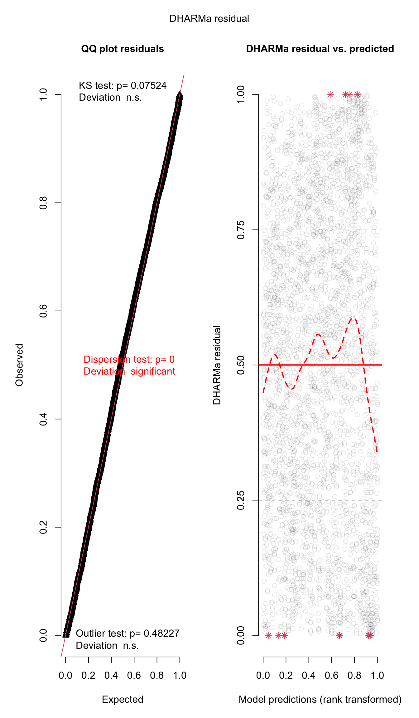

Past versions of unnamed-chunk-41-4.png

Version	Author	Date
a7bae31	MartinGarlovsky	2024-10-09

>>>> Results

car::Anova(viability_m2, type = "3") %>% 
  broom::tidy() %>% 
  #write_csv("output/anova_tables/viability_t30.csv") %>% # save anova table for supp. tables
  as_tibble() %>% 
  kable(digits = 3, 
        caption = 'Analysis of Deviance Table (Type III Wald chisquare tests)') %>% 
  kable_styling(full_width = FALSE)

Analysis of Deviance Table (Type III Wald chisquare tests)

term	statistic	df	p.value
(Intercept)	77.698	1	0.000
mito	7.119	2	0.028
nuclear	0.545	2	0.761
age	58.101	1	0.000
days	3.514	1	0.061
block	15.118	1	0.000
mito:nuclear	3.759	4	0.440
mito:age	0.853	2	0.653
nuclear:age	6.022	2	0.049
mito:nuclear:age	1.778	4	0.777

#summary(viability_m2)

# posthoc tests
bind_rows(emmeans(viability_m2, pairwise ~ mito, adjust = "tukey")$contrasts %>% broom::tidy() %>%
            rename(p.value = adj.p.value),
          emmeans(viability_m2, pairwise ~ block, adjust = "tukey")$contrasts %>% broom::tidy(),
          emmeans(viability_m2, pairwise ~ age | nuclear, adjust = "tukey")$contrasts %>% broom::tidy(),
          emmeans(viability_m2, pairwise ~ nuclear | age, adjust = "tukey")$contrasts %>% broom::tidy() %>%
            rename(p.value = adj.p.value)) %>% 
  mutate(p.val = ifelse(p.value < 0.001, '< 0.001', round(p.value, 3))) %>% 
  select(-p.value, -term) %>% relocate(age, .before = contrast) %>% 
  kable(digits = 3, 
        caption = 'Posthoc Tukey tests to compare which groups differ') %>% 
  kable_styling(full_width = FALSE) %>%
  kableExtra::group_rows("Mitochondria", 1, 3) %>%
  kableExtra::group_rows("Block", 4, 4) %>%
  kableExtra::group_rows("Age", 5, 7) %>%
  kableExtra::group_rows("Nuclear - old", 8, 10) %>%
  kableExtra::group_rows("Nuclear - young", 11, 13)

Posthoc Tukey tests to compare which groups differ

age	contrast	null.value	estimate	std.error	df	statistic	nuclear	p.val
Mitochondria
NA	A - B	0	-0.182	0.084	Inf	-2.158	NA	0.079
NA	A - C	0	-0.208	0.086	Inf	-2.412	NA	0.042
NA	B - C	0	-0.026	0.087	Inf	-0.297	NA	0.953
Block
NA	block1 - block2	0	0.270	0.069	Inf	3.888	NA	< 0.001
Age
NA	young - old	0	0.791	0.119	Inf	6.647	A	< 0.001
NA	young - old	0	0.498	0.133	Inf	3.741	B	< 0.001
NA	young - old	0	0.399	0.118	Inf	3.376	C	< 0.001
Nuclear - old
young	A - B	0	0.170	0.107	Inf	1.584	NA	0.253
young	A - C	0	0.156	0.107	Inf	1.461	NA	0.31
young	B - C	0	-0.013	0.106	Inf	-0.124	NA	0.992
Nuclear - young
old	A - B	0	-0.123	0.139	Inf	-0.889	NA	0.647
old	A - C	0	-0.236	0.126	Inf	-1.874	NA	0.146
old	B - C	0	-0.113	0.139	Inf	-0.813	NA	0.695

>>>>> Reaction norms

sperm_stress_norm <- emmeans(viability_m2, ~ mito * nuclear * age, type = 'response') %>% as_tibble() %>% 
  ggplot(aes(x = nuclear, y = prob, fill = mito)) +
  geom_line(aes(group = mito, colour = mito), position = position_dodge(width = .5)) +
  # geom_errorbar(aes(ymin = asymp.LCL, ymax = asymp.UCL),
  #               width = .25, position = position_dodge(width = .5)) +
  geom_point(size = 3, pch = 21, position = position_dodge(width = .5)) +
  labs(y = 'Sperm viability (EMM)') +
  scale_colour_manual(values = met3) +
  scale_fill_manual(values = met3) +
  facet_wrap(~ age) +
  theme_bw() + 
  theme() + 
  NULL

sperm_stress_norm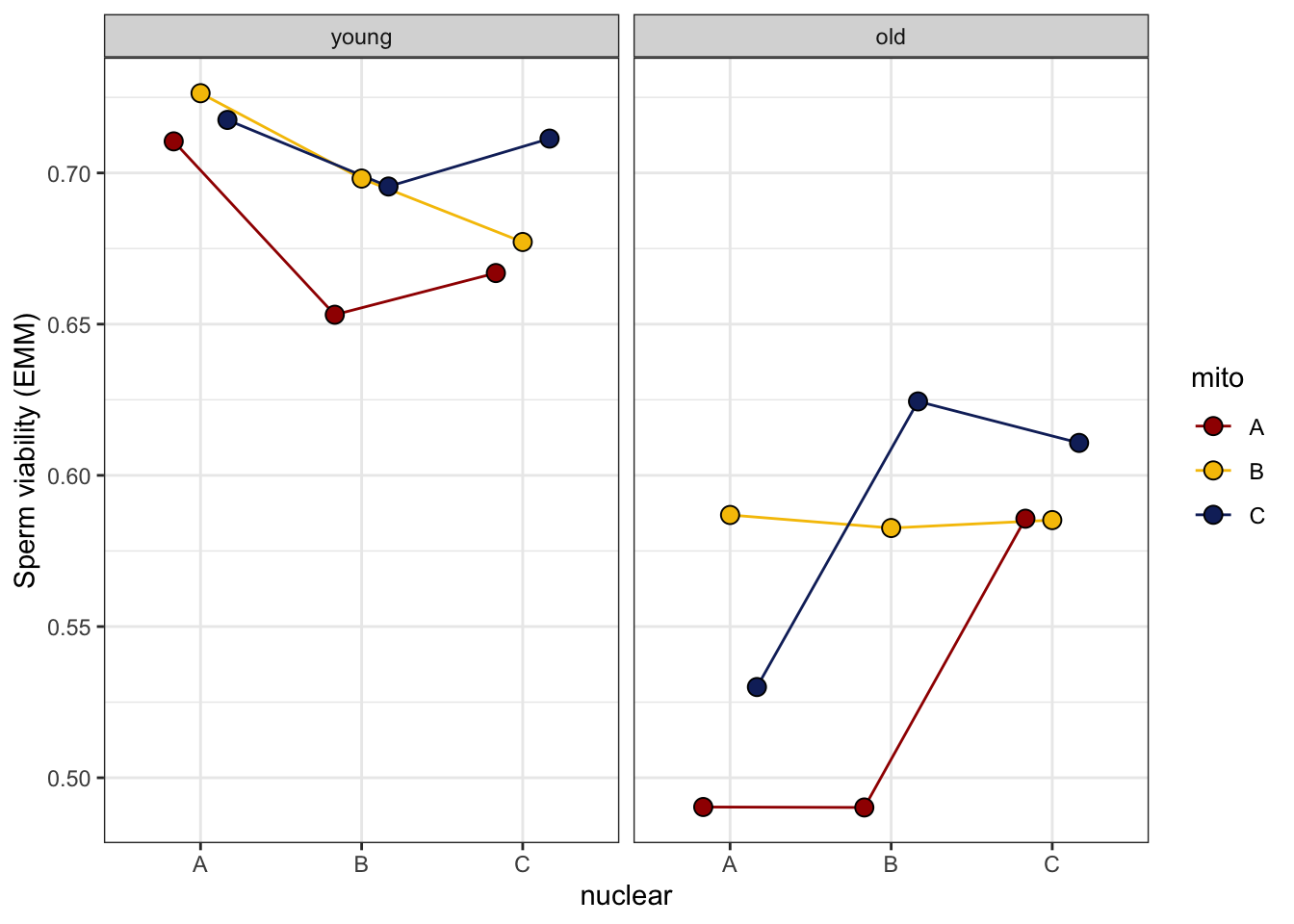

Past versions of unnamed-chunk-43-1.png

Version	Author	Date
a7bae31	MartinGarlovsky	2024-10-09

>>>>> Raw data and means

sperm_stress_raw <- emmeans(viability_m2, ~ mito * nuclear * age, type = 'response') %>% as_tibble() %>% 
  ggplot(aes(x = nuclear, y = prob, fill = mito)) +
  geom_jitter(data = spvfilt_treat %>% 
               group_by(mito, nuclear, age, treatment, male_ID) %>% 
               summarise(viability = mean(viability)),
              aes(y = viability, colour = mito),
               position = position_jitterdodge(dodge.width = .5, jitter.width = .1),
              size = 0.75, alpha = .1) +
  geom_jitter(data = spvfilt_treat %>% 
                group_by(LINE, age) %>% 
                summarise(mn = mean(viability)) %>% 
                separate(LINE, into = c("mito", "nuclear", NA), sep = "(?<=.)", remove = FALSE),
              aes(y = mn, colour = mito),
              position = position_jitterdodge(dodge.width = .5, jitter.width = .1),
              alpha = .85, size = 2) +
  geom_errorbar(aes(ymin = asymp.LCL, ymax = asymp.UCL), 
                width = .25, position = position_dodge(width = .5)) +
  geom_point(size = 3, pch = 21, position = position_dodge(width = .5)) +
  labs(y = 'Sperm viability (EMM ± 95% CIs)') +
  scale_colour_manual(values = met3) +
  scale_fill_manual(values = met3) +
  facet_wrap(~ age) +
  theme_bw() + 
  theme() + 
  geom_text(data = spvfilt_control %>% 
              group_by(mito, nuclear, age) %>% 
              summarise(N = n_distinct(male_ID)), 
            aes(y = -0.04, label = N), 
            size = 2, position = position_dodge(width = .5)) + 
  #ggsave('figures/sperm_stress_raw.pdf', height = 4, width = 8, dpi = 600, useDingbats = FALSE) +
  NULL

sperm_stress_raw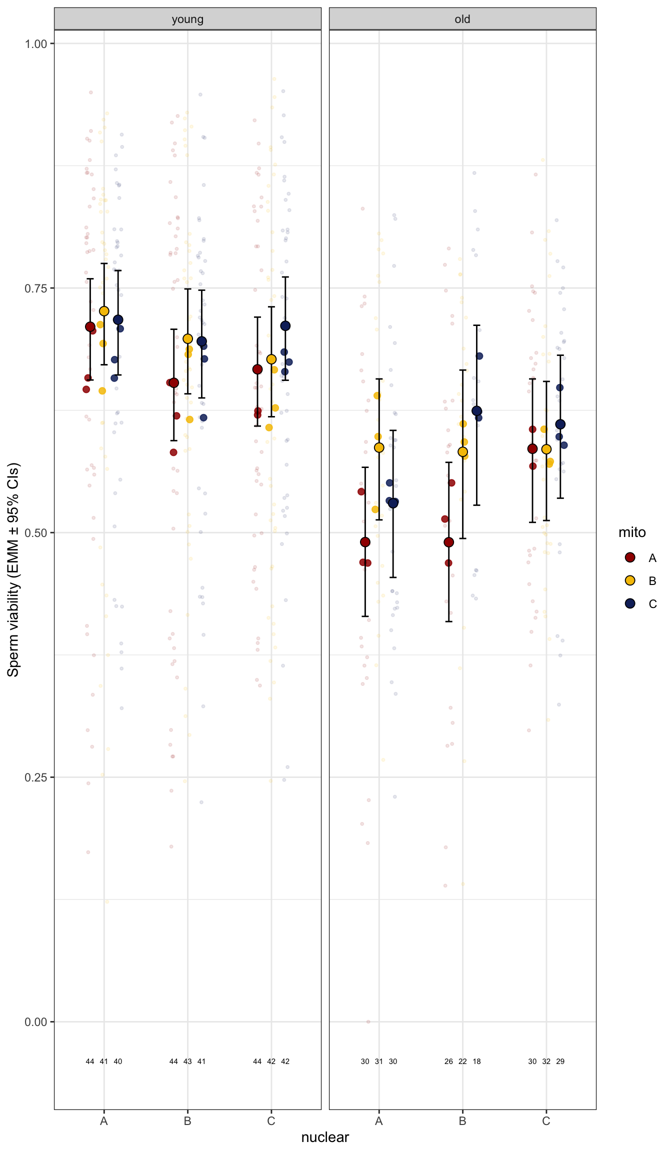

Past versions of unnamed-chunk-44-1.png

Version	Author	Date
a7bae31	MartinGarlovsky	2024-10-09

Matched vs. mismatched

stress_coevo <- glmer(cbind(live, dead) ~ coevolved * age + days + block + (age|LINE) + (1|male_ID) + (1|OLRE),
                      data = spvfilt_treat, family = 'binomial')

car::Anova(stress_coevo, type = "3")

Analysis of Deviance Table (Type III Wald chisquare tests)

Response: cbind(live, dead)
                Chisq Df Pr(>Chisq)    
(Intercept)   75.6518  1  < 2.2e-16 ***
coevolved      0.1516  1  0.6970370    
age           56.4580  1  5.741e-14 ***
days           3.5747  1  0.0586647 .  
block         15.0434  1  0.0001051 ***
coevolved:age  0.5181  1  0.4716464    
---
Signif. codes:  0 '***' 0.001 '**' 0.01 '*' 0.05 '.' 0.1 ' ' 1

Mito-type analysis

viability_m2_snp <- glmer(cbind(live, dead) ~ mito_snp * nuclear * age +  days + block + 
                            (1 + age|LINE) + (1|male_ID) + (1|OLRE),
                          data = spvfilt_treat, family = 'binomial',
                      control = glmerControl(optimizer = "bobyqa", optCtrl = list(maxfun = 50000)))

car::Anova(viability_m2_snp, type = "3")

Analysis of Deviance Table (Type III Wald chisquare tests)

Response: cbind(live, dead)
                       Chisq Df Pr(>Chisq)    
(Intercept)          28.9303  1  7.503e-08 ***
mito_snp             11.0643  8    0.19808    
nuclear               0.5764  2    0.74962    
age                   5.6219  1    0.01774 *  
days                  3.6522  1    0.05600 .  
block                15.2930  1  9.206e-05 ***
mito_snp:nuclear      2.0731  7    0.95568    
mito_snp:age          0.9689  8    0.99844    
nuclear:age           2.4954  2    0.28716    
mito_snp:nuclear:age  2.8611  7    0.89755    
---
Signif. codes:  0 '***' 0.001 '**' 0.01 '*' 0.05 '.' 0.1 ' ' 1

Combined plots

sperm_diffs_norm <- emmeans(viability_m1, ~ mito * nuclear * age, type = 'response') %>% as_tibble() %>% 
  ggplot(aes(x = nuclear, y = prob, fill = mito)) +
  geom_line(aes(group = mito, colour = mito), position = position_dodge(width = .5)) +
  # geom_errorbar(aes(ymin = asymp.LCL, ymax = asymp.UCL),
  #               width = .25, position = position_dodge(width = .5)) +
  geom_point(size = 3, pch = 23, position = position_dodge(width = .5)) +
  # after stress
  geom_line(data = emmeans(viability_m2, ~ mito * nuclear * age, type = 'response') %>% as_tibble(),
            aes(group = mito, colour = mito), position = position_dodge(width = .5)) +
  # geom_errorbar(data = emmeans(viability_m2, ~ mito * nuclear * age, type = 'response') %>% as_tibble(),
  #               aes(ymin = asymp.LCL, ymax = asymp.UCL),
  #               width = .25, position = position_dodge(width = .5)) +
  geom_point(data = emmeans(viability_m2, ~ mito * nuclear * age, type = 'response') %>% as_tibble(),
             aes(fill = mito), size = 3, pch = 22, position = position_dodge(width = .5)) + 
  labs(y = 'Sperm viability (EMM)') +
  scale_colour_manual(values = met3) +
  scale_fill_manual(values = met3) +
  facet_wrap(~ age) +
  theme_bw() + 
  theme() + 
  NULL

sperm_diffs_norm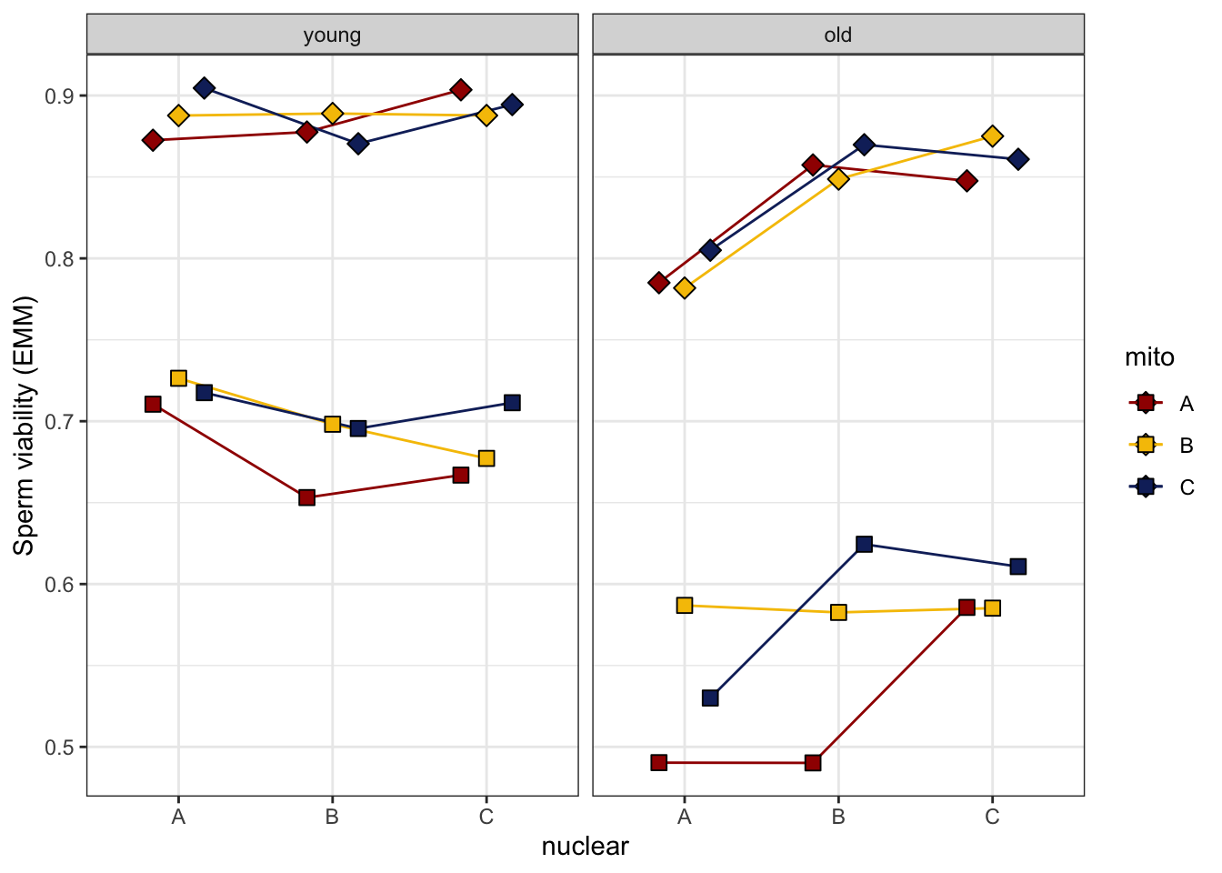

Past versions of unnamed-chunk-47-1.png

Version	Author	Date
a7bae31	MartinGarlovsky	2024-10-09

# bind_rows(
#   emmeans(viability_m1, ~ mito * nuclear * age, type = 'response') %>% as_tibble() %>% mutate(stage = "t0"),
#   emmeans(viability_m2, ~ mito * nuclear * age, type = 'response') %>% as_tibble() %>% mutate(stage = "t30")) %>%
#   ggplot(aes(x = nuclear, y = prob, fill = mito, shape = stage)) +
#   geom_errorbar(aes(ymin = asymp.LCL, ymax = asymp.UCL), position = position_dodge(width = .5), width = .5) +
#   geom_line(aes(group = interaction(mito, stage), colour = mito), position = position_dodge(width = .5)) +
#   geom_point(size = 3, position = position_dodge(width = .5)) +
#   labs(y = 'No. progeny (EMM)') +
#   scale_colour_manual(values = met3) +
#   scale_fill_manual(values = met3) +
#   scale_shape_manual(values = c(23, 22)) + 
#   facet_wrap(~ age) +
#   theme_bw() + 
#   theme() + 
#   NULL

>> Sperm quality

For the analysis of sperm quality we calculated the mean difference in sperm viability between treated and control for each male. In the plots below lines connect the mean measurements for each male, showing the overall average decline in viability after stress treatment.

# calculate difference in viability between treatment/control for each male
viability_diff <- sperm_vib_filt %>%
  group_by(treatment, mito, mito_snp, nuclear, coevolved, LINE, age, male_ID, block, days) %>% 
  summarise(mn_vib = mean(viability)) %>% #filter(male_ID == 1) %>% 
  pivot_wider(names_from = treatment, 
              values_from = mn_vib) %>% 
  mutate(diff = t - c)

>>> Young males

viability_diff %>% pivot_longer(cols = c(c, t)) %>% filter(age == "young") %>% 
  ggplot(aes(x = name, y = value)) + 
  geom_line(aes(group = male_ID, colour = mito)) +
  scale_colour_manual(values = met3) +
  facet_grid(mito ~ nuclear) +
  NULL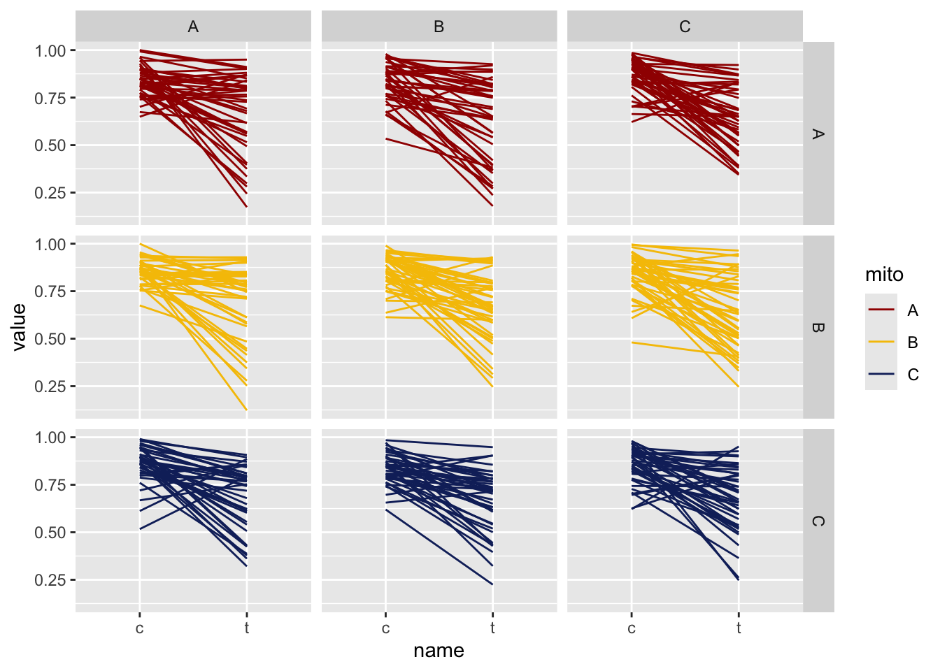

Past versions of unnamed-chunk-49-1.png

Version	Author	Date
a7bae31	MartinGarlovsky	2024-10-09

>>> Old males

viability_diff %>% pivot_longer(cols = c(c, t)) %>% filter(age == "old") %>% 
  ggplot(aes(x = name, y = value)) + 
  geom_line(aes(group = male_ID, colour = mito)) +
  scale_colour_manual(values = met3) +
  facet_grid(mito ~ nuclear) +
  NULL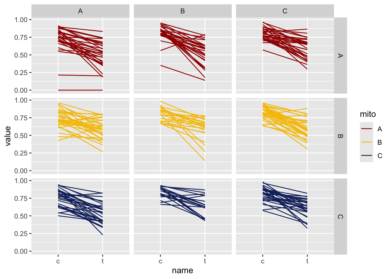

Past versions of unnamed-chunk-50-1.png

Version	Author	Date
a7bae31	MartinGarlovsky	2024-10-09

hist(viability_diff$diff)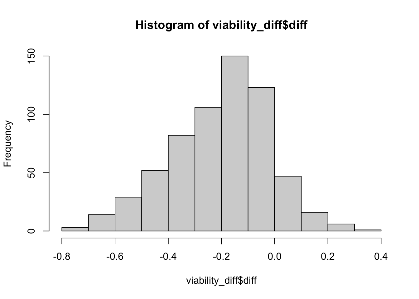

Past versions of unnamed-chunk-51-1.png

Version	Author	Date
a7bae31	MartinGarlovsky	2024-10-09

vib_diff_test <- lmerTest::lmer(diff ~ mito * nuclear * age + block + days + (1 + age|LINE), 
                                data = viability_diff)

>>> Check diagnostics

performance::check_model(vib_diff_test)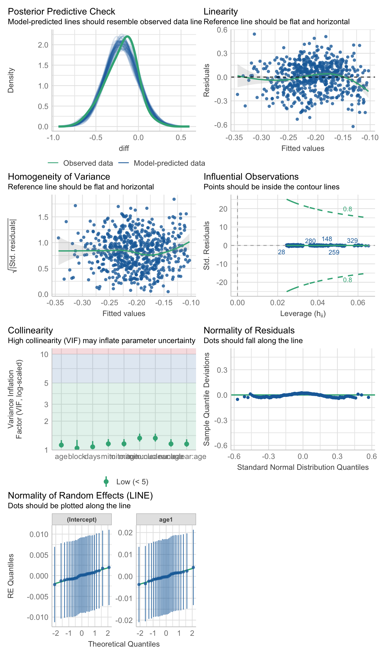

Past versions of unnamed-chunk-52-1.png

Version	Author	Date
0ffce9c	MartinGarlovsky	2024-10-10
a7bae31	MartinGarlovsky	2024-10-09

testDispersion(vib_diff_test)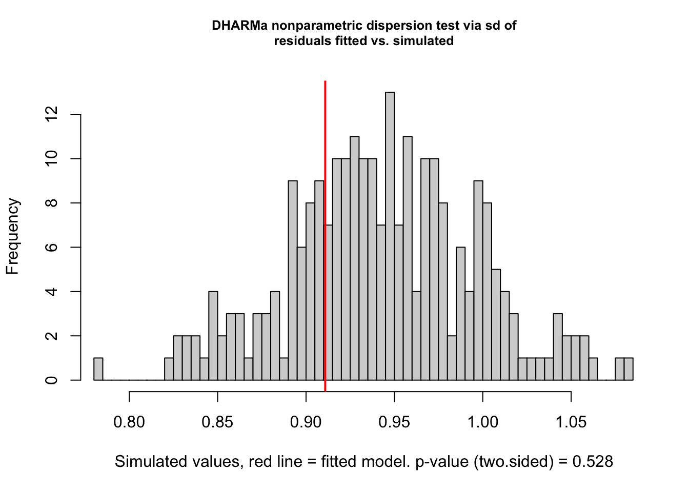

Past versions of unnamed-chunk-53-1.png

Version	Author	Date
a7bae31	MartinGarlovsky	2024-10-09

    DHARMa nonparametric dispersion test via sd of residuals fitted vs.
    simulated

data:  simulationOutput
dispersion = 0.96613, p-value = 0.528
alternative hypothesis: two.sided

simulationOutput <- simulateResiduals(fittedModel = vib_diff_test, plot = FALSE)
hist(residuals(simulationOutput))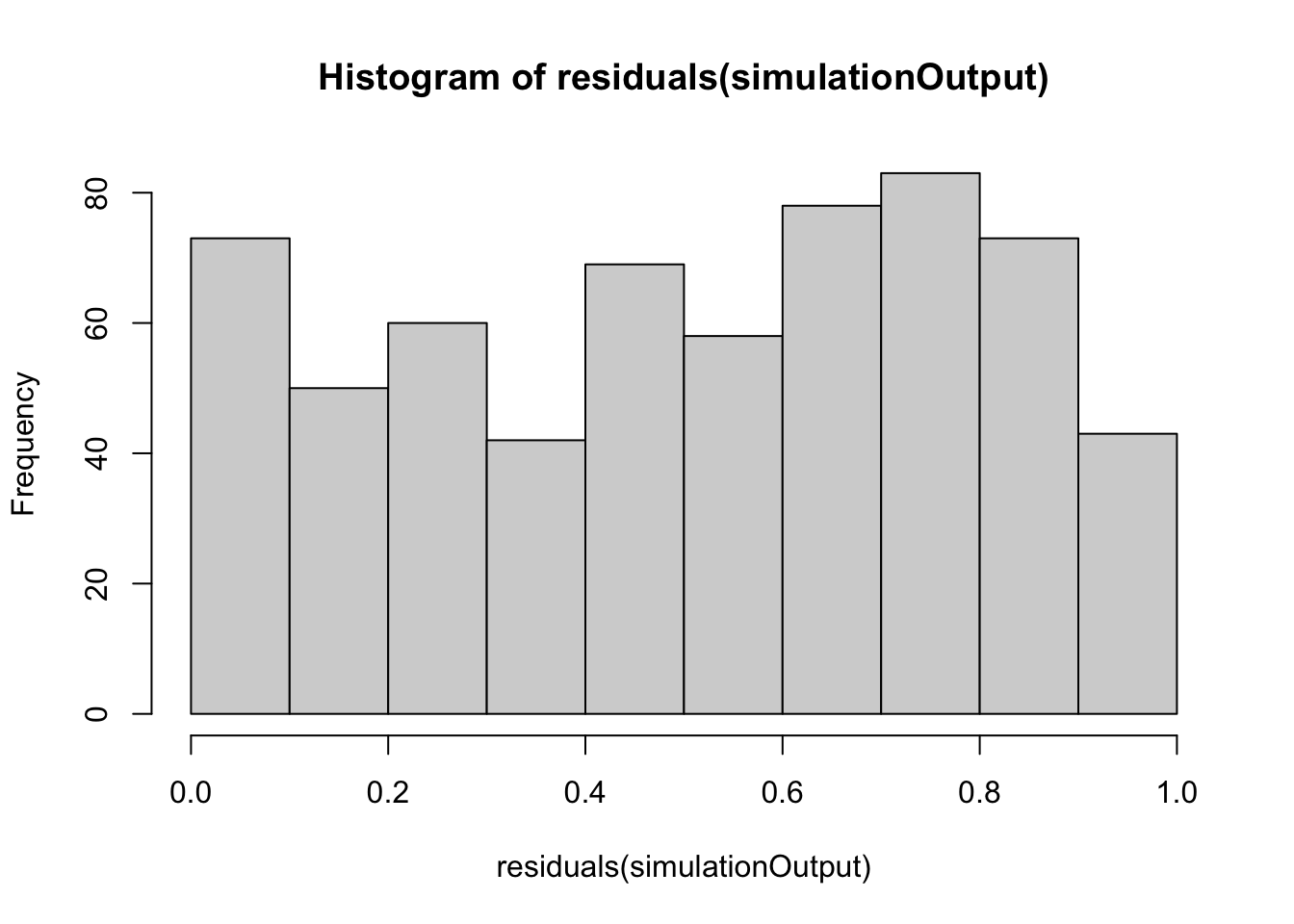

Past versions of unnamed-chunk-53-2.png

Version	Author	Date
a7bae31	MartinGarlovsky	2024-10-09

hist(residuals(simulationOutput, quantileFunction = qnorm, outlierValues = c(-7,7)))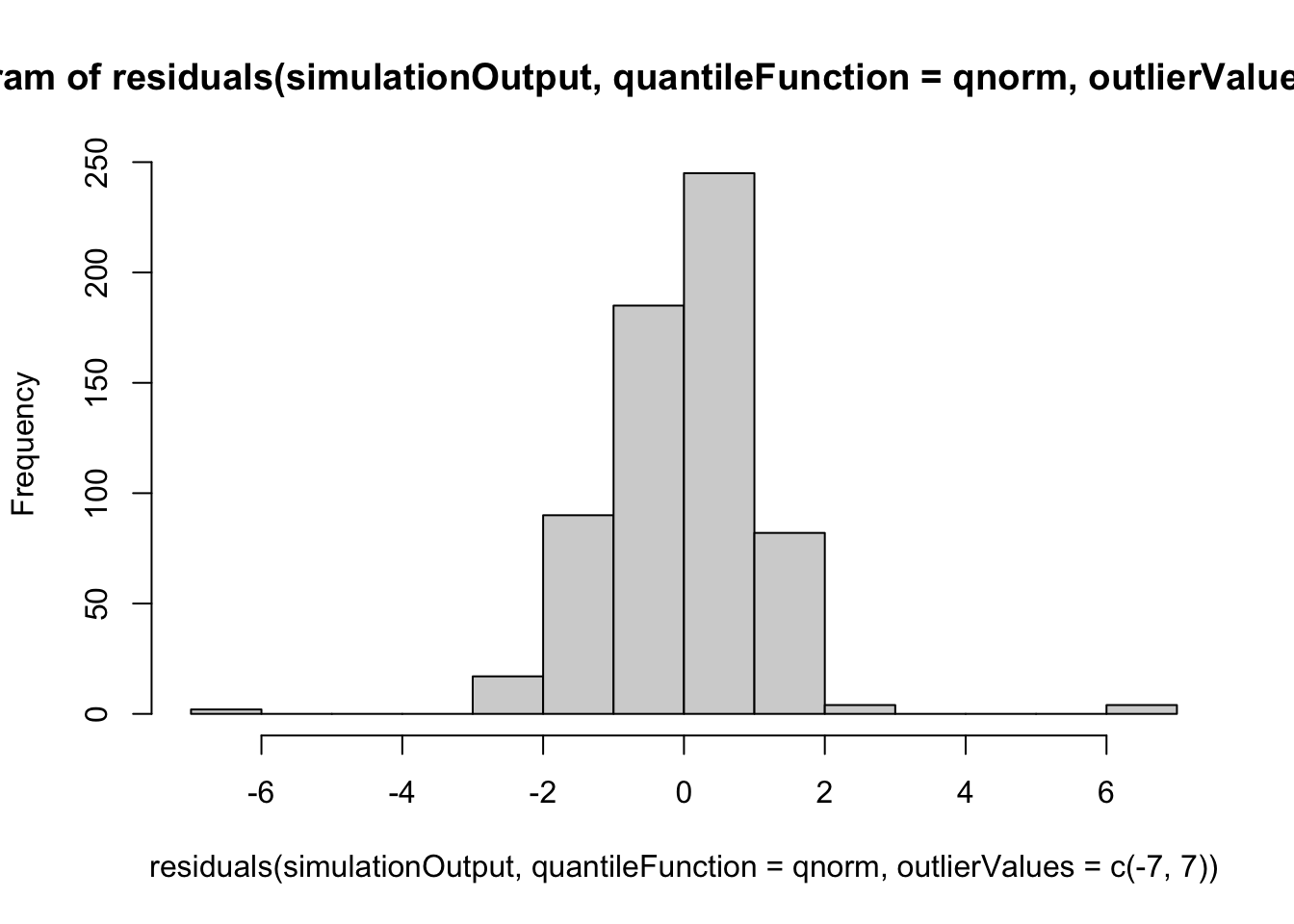

Past versions of unnamed-chunk-53-3.png

Version	Author	Date
a7bae31	MartinGarlovsky	2024-10-09

plot(simulationOutput)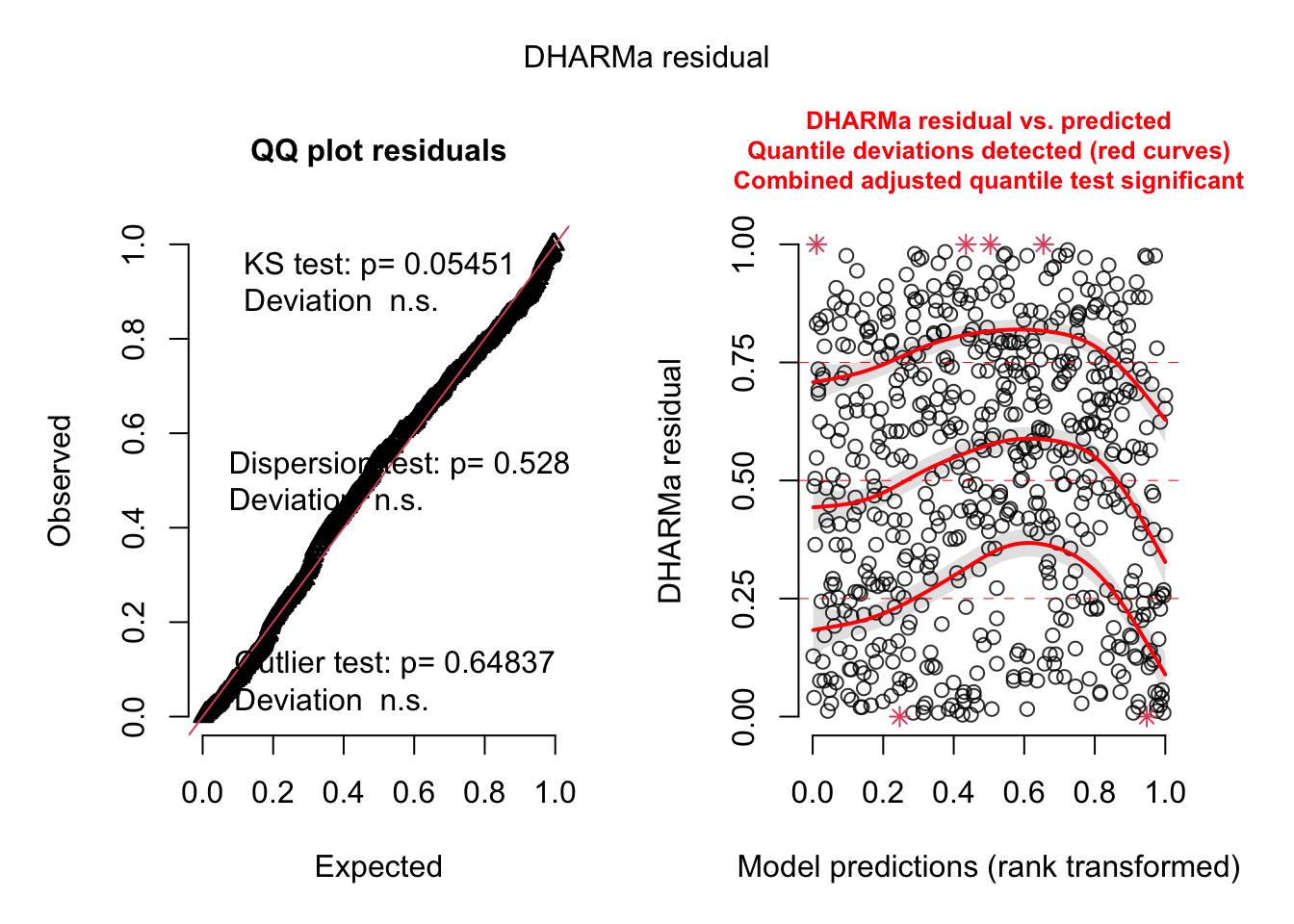

Past versions of unnamed-chunk-53-4.png

Version	Author	Date
a7bae31	MartinGarlovsky	2024-10-09

>>> Results

anova(vib_diff_test, type = "III", ddf = "Kenward-Roger") %>% 
  broom::tidy() %>% 
  as_tibble() %>% 
  #write_csv("output/anova_tables/sperm_quality.csv") %>% # save anova table for supp. tables
  kable(digits = 3, 
        caption = 'Type III Analysis of Variance Table with Kenward-Roger`s method') %>% 
  kable_styling(full_width = FALSE)

Type III Analysis of Variance Table with Kenward-Roger`s method

term	sumsq	meansq	NumDF	DenDF	statistic	p.value
mito	0.128	0.064	2	18.585	1.894	0.178
nuclear	0.130	0.065	2	18.471	1.915	0.176
age	0.315	0.315	1	22.638	9.312	0.006
block	0.345	0.345	1	579.154	10.204	0.001
days	0.255	0.255	1	576.522	7.549	0.006
mito:nuclear	0.172	0.043	4	18.333	1.271	0.317
mito:age	0.025	0.013	2	18.551	0.376	0.692
nuclear:age	0.030	0.015	2	18.432	0.447	0.646
mito:nuclear:age	0.093	0.023	4	18.331	0.686	0.611

#summary(vib_diff_test)

# posthoc tests
bind_rows(emmeans(vib_diff_test, pairwise ~ age, adjust = "tukey")$contrasts %>% broom::tidy(),
          emmeans(vib_diff_test, pairwise ~ block, adjust = "tukey")$contrasts %>% broom::tidy()) %>% 
  kable(digits = 3, 
        caption = 'Posthoc Tukey tests to compare which groups differ. Results are averaged over the levels of: mito, nuclear, age, block') %>% 
  kable_styling(full_width = FALSE) %>%
  kableExtra::group_rows("Age", 1, 1) %>%
  kableExtra::group_rows("Block", 2, 2)

Posthoc Tukey tests to compare which groups differ. Results are averaged over the levels of: mito, nuclear, age, block

term	contrast	null.value	estimate	std.error	df	statistic	p.value
Age
age	young - old	0	0.050	0.016	22.638	3.051	0.006
Block
block	block1 - block2	0	0.048	0.015	579.154	3.194	0.001

emtrends(vib_diff_test, ~ days, var = "days") %>% broom::tidy() %>% 
  kable(digits = 3, 
        caption = 'Posthoc Tukey tests for days effect. Results are averaged over the levels of: mito, nuclear, age, block') %>% 
  kable_styling(full_width = FALSE)

Posthoc Tukey tests for days effect. Results are averaged over the levels of: mito, nuclear, age, block

days	days.trend	std.error	df	statistic	p.value
3.738	-0.01	0.004	576.522	-2.747	0.006

>>>> Reaction norms

sperm_qual_norm <- emmeans(vib_diff_test, ~ mito * nuclear * age) %>% as_tibble() %>% 
  ggplot(aes(x = nuclear, y = emmean, fill = mito)) +
  geom_line(aes(group = mito, colour = mito), position = position_dodge(width = .5)) +
  # geom_errorbar(aes(ymin = lower.CL, ymax = upper.CL),
  #               width = .25, position = position_dodge(width = .5)) +
  geom_point(size = 3, pch = 21, position = position_dodge(width = .5)) +
  labs(y = 'Sperm viability (EMM)') +
  scale_colour_manual(values = met3) +
  scale_fill_manual(values = met3) +
  facet_wrap(~ age) +
  theme_bw() + 
  theme() + 
  NULL

sperm_qual_norm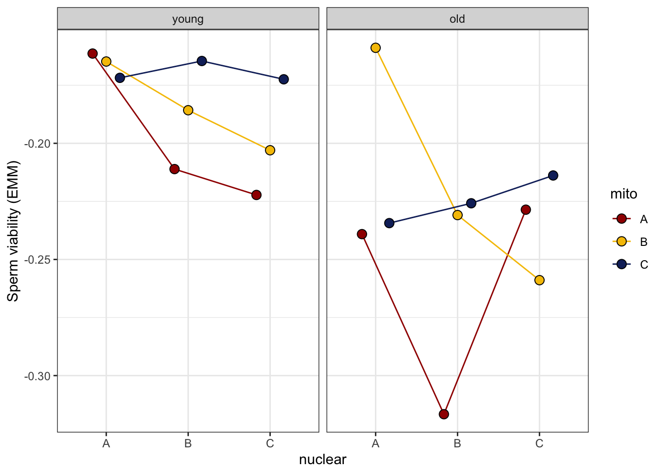

Past versions of unnamed-chunk-55-1.png

Version	Author	Date
a7bae31	MartinGarlovsky	2024-10-09

>>> Matched vs. mismatched

vib_diff_coevo <- lmerTest::lmer(diff ~ coevolved * age + block + days + (age|LINE), 
                                 data = viability_diff,
                                 na.action = 'na.fail')

anova(vib_diff_coevo, type = "III", ddf = "Kenward-Roger")

Type III Analysis of Variance Table with Kenward-Roger's method
               Sum Sq Mean Sq NumDF  DenDF F value   Pr(>F)   
coevolved     0.01983 0.01983     1  24.82  0.5866 0.450964   
age           0.27915 0.27915     1  29.18  8.2593 0.007489 **
block         0.33197 0.33197     1 586.41  9.8219 0.001811 **
days          0.25758 0.25758     1 579.82  7.6210 0.005952 **
coevolved:age 0.00253 0.00253     1  24.85  0.0748 0.786719   
---
Signif. codes:  0 '***' 0.001 '**' 0.01 '*' 0.05 '.' 0.1 ' ' 1

>>> Mito-type analysis

vib_diff_snp <- lmerTest::lmer(diff ~ mito_snp * nuclear * age + block + days + (1 + age|LINE), 
                               data = viability_diff)

anova(vib_diff_snp, type = "III", ddf = "Kenward-Roger")

Type III Analysis of Variance Table with Kenward-Roger's method
                      Sum Sq Mean Sq NumDF  DenDF F value   Pr(>F)   
mito_snp             0.29901 0.03738     8   9.09  1.0899 0.445593   
nuclear              0.07678 0.03839     2   8.96  1.1188 0.368350   
age                  0.38706 0.38706     1  10.43 11.2829 0.006848 **
block                0.34418 0.34418     1 575.40 10.0328 0.001619 **
days                 0.25922 0.25922     1 575.16  7.5564 0.006168 **
mito_snp:nuclear     0.10879 0.01554     7   9.08  0.4530 0.845633   
mito_snp:age         0.23540 0.02942     8   9.09  0.8580 0.579924   
nuclear:age          0.01427 0.00714     2   8.95  0.2079 0.816073   
mito_snp:nuclear:age 0.14458 0.02065     7   9.08  0.6020 0.742017   
---
Signif. codes:  0 '***' 0.001 '**' 0.01 '*' 0.05 '.' 0.1 ' ' 1

> Sperm metabolic rate

We measured the metabolic rate of sperm dissected from seminal vesicles using NAD(P)H autofluorescence lifetime imaging (FLIM). Specifically, here we use parameter a2 (see online supplementary material for detailed methods).

Looking at the data there is a clear outlier in old males where a2 > 50. We will analyse the data including and excluding this outlier.

sperm_met %>% 
  group_by(mito, nuclear, age) %>% 
  summarise(mn = mean(a2),
            se = sd(a2)/sqrt(n()),
            s95 = se * 1.96) %>% 
  ggplot(aes(x = nuclear, y = mn, fill = mito)) +
  geom_point(data = sperm_met,
             aes(y = a2, colour = mito), alpha = .25,
             position = position_jitterdodge(dodge.width = .5, jitter.width = .1)) +
  geom_errorbar(aes(ymin = mn - s95, ymax = mn + s95), 
                width = .25, position = position_dodge(width = .5)) +
  geom_point(size = 3, pch = 21, position = position_dodge(width = .5)) +
  labs(y = 'a2') +
  facet_wrap(~ age, scales = 'free_x') +
  scale_colour_manual(values = met3) +
  scale_fill_manual(values = met3) +
  theme_bw() + 
  theme() + 
  NULL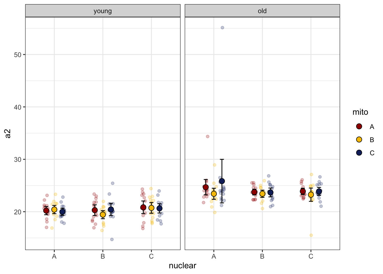

Past versions of unnamed-chunk-58-1.png

Version	Author	Date
a7bae31	MartinGarlovsky	2024-10-09

>> Analysis

hist(sperm_met$p.a2, breaks = 50)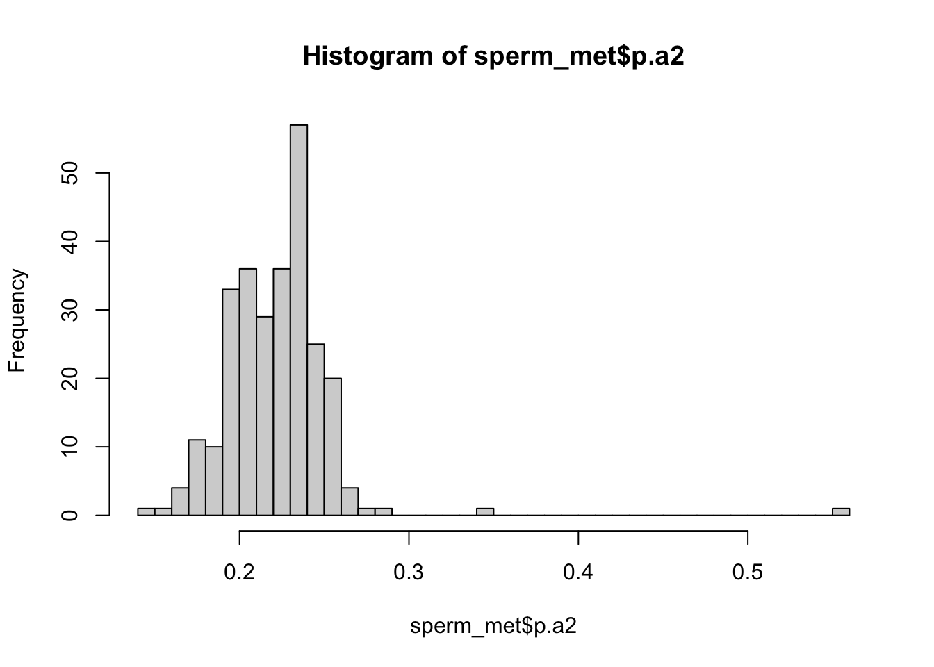

Past versions of unnamed-chunk-59-1.png

Version	Author	Date
a7bae31	MartinGarlovsky	2024-10-09

>>> With outlier

met_mod_outlier_test <- lmerTest::lmer(p.a2 ~ mito * nuclear * age + (1 + age|LINE),
                                       data = sperm_met, REML = TRUE)

anova(met_mod_outlier_test, type = "III", ddf = "Kenward-Roger")

Type III Analysis of Variance Table with Kenward-Roger's method
                   Sum Sq  Mean Sq NumDF  DenDF  F value    Pr(>F)    
mito             0.001762 0.000881     2 17.996   1.2674    0.3055    
nuclear          0.001419 0.000710     2 17.996   1.0206    0.3803    
age              0.086787 0.086787     1 17.996 124.8329 1.584e-09 ***
mito:nuclear     0.000415 0.000104     4 17.995   0.1492    0.9609    
mito:age         0.000956 0.000478     2 17.995   0.6876    0.5155    
nuclear:age      0.002506 0.001253     2 17.995   1.8020    0.1935    
mito:nuclear:age 0.002388 0.000597     4 17.994   0.8586    0.5072    
---
Signif. codes:  0 '***' 0.001 '**' 0.01 '*' 0.05 '.' 0.1 ' ' 1

>>> Without outlier

met_mod_test <- lmerTest::lmer(p.a2 ~ mito * nuclear * age + (1 + age|LINE),
                                       data = sperm_met %>% filter(a2 <= 30), REML = TRUE)

>>>> Check diagnostics

performance::check_model(met_mod_outlier_test)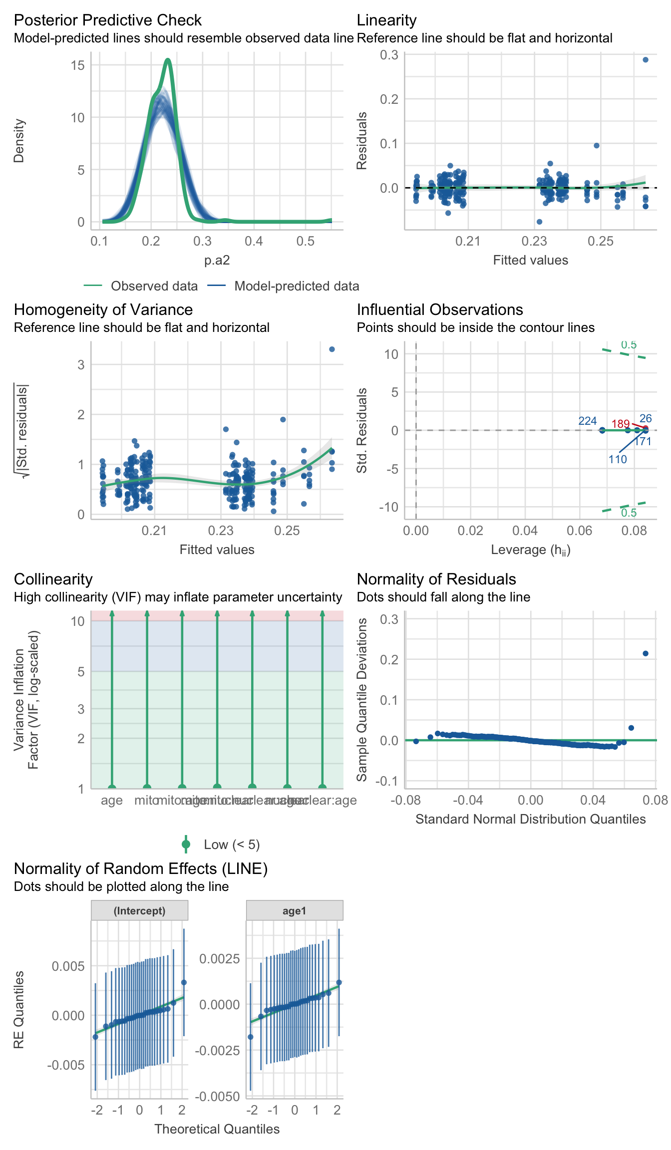

Past versions of unnamed-chunk-62-1.png

Version	Author	Date
0ffce9c	MartinGarlovsky	2024-10-10
a7bae31	MartinGarlovsky	2024-10-09

testDispersion(met_mod_outlier_test)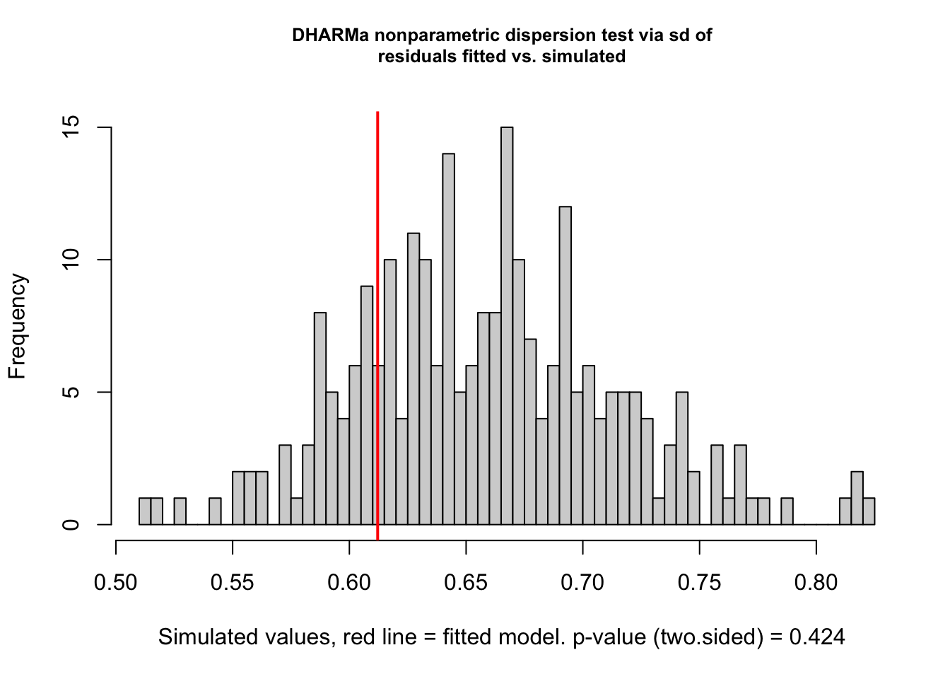

Past versions of unnamed-chunk-63-1.png

Version	Author	Date
a7bae31	MartinGarlovsky	2024-10-09

    DHARMa nonparametric dispersion test via sd of residuals fitted vs.
    simulated

data:  simulationOutput
dispersion = 0.92929, p-value = 0.424
alternative hypothesis: two.sided

simulationOutput <- simulateResiduals(fittedModel = met_mod_outlier_test, plot = FALSE)
hist(residuals(simulationOutput))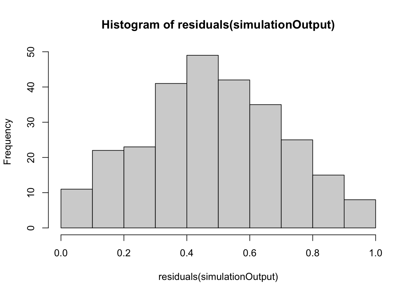

Past versions of unnamed-chunk-63-2.png

Version	Author	Date
a7bae31	MartinGarlovsky	2024-10-09

hist(residuals(simulationOutput, quantileFunction = qnorm, outlierValues = c(-7,7)))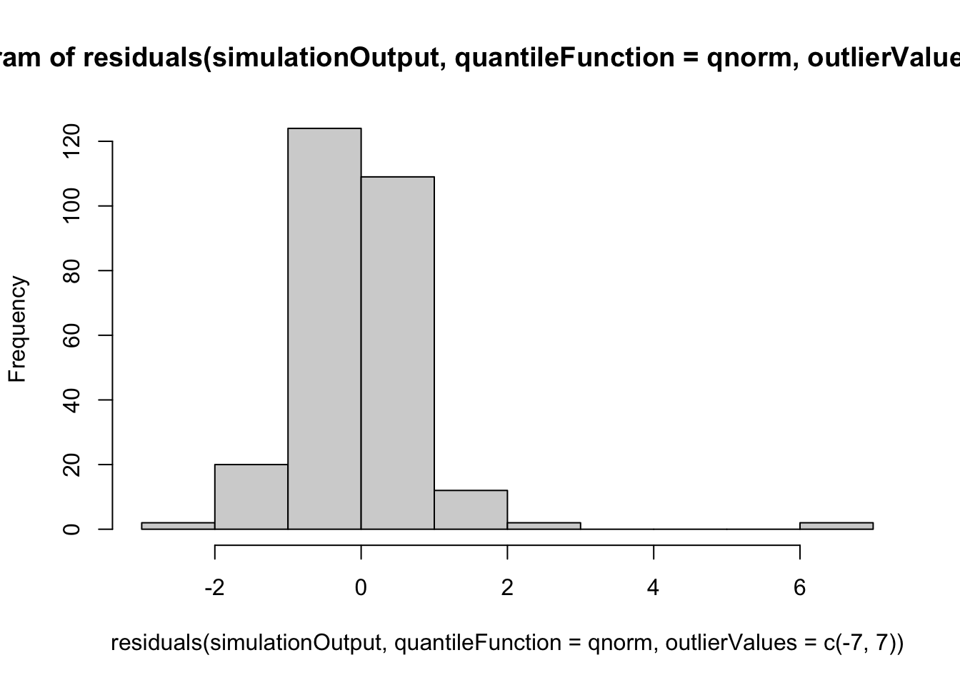

Past versions of unnamed-chunk-63-3.png

Version	Author	Date
a7bae31	MartinGarlovsky	2024-10-09

plot(simulationOutput)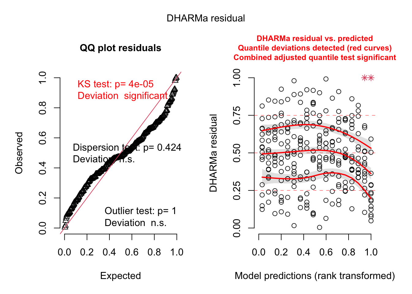

Past versions of unnamed-chunk-63-4.png

Version	Author	Date
a7bae31	MartinGarlovsky	2024-10-09

>> Results

anova(met_mod_test, type = "III", ddf = "Kenward-Roger") %>% 
  broom::tidy() %>% 
  as_tibble() #%>% write_csv("output/anova_tables/sperm_metabolism.csv") %>% # save anova table for supp. tables

# A tibble: 7 × 7
  term                 sumsq    meansq NumDF DenDF statistic  p.value
                                  
1 mito             0.000699  0.000350      2  18.0     1.16  3.37e- 1
2 nuclear          0.000625  0.000313      2  18.0     1.04  3.75e- 1
3 age              0.0726    0.0726        1  18.0   240.    7.51e-12
4 mito:nuclear     0.000341  0.0000852     4  18.0     0.282 8.86e- 1
5 mito:age         0.0000876 0.0000438     2  18.0     0.145 8.66e- 1
6 nuclear:age      0.000535  0.000268      2  18.0     0.886 4.29e- 1
7 mito:nuclear:age 0.000611  0.000153      4  18.0     0.506 7.32e- 1

met_emm <- emmeans(met_mod_test, ~ mito * nuclear * age)

emmeans(met_mod_test, pairwise ~ age, adjust = "tukey")

$emmeans
 age   emmean      SE   df lower.CL upper.CL
 young  0.203 0.00153 18.0    0.200    0.207
 old    0.237 0.00150 17.9    0.234    0.240

Results are averaged over the levels of: mito, nuclear 
Degrees-of-freedom method: kenward-roger 
Confidence level used: 0.95 

$contrasts
 contrast    estimate      SE df t.ratio p.value
 young - old  -0.0334 0.00215 18 -15.503  <.0001

Results are averaged over the levels of: mito, nuclear 
Degrees-of-freedom method: kenward-roger 

>>> Reaction norms

sperm_met_norm <- emmeans(met_mod_test, ~ mito * nuclear * age) %>% as_tibble() %>% 
  ggplot(aes(x = nuclear, y = emmean, fill = mito)) +
  geom_line(aes(group = mito, colour = mito), position = position_dodge(width = .5)) +
  # geom_errorbar(aes(ymin = lower.CL, ymax = upper.CL), 
  #               width = .25, position = position_dodge(width = .5)) +
  geom_point(size = 3, pch = 21, position = position_dodge(width = .5)) +
  labs(y = 'Sperm metabolic rate, a2 (EMM)') +
  scale_colour_manual(values = met3) +
  scale_fill_manual(values = met3) +
  facet_wrap(~ age) +
  theme_bw() + 
  theme() + 
  NULL

sperm_met_norm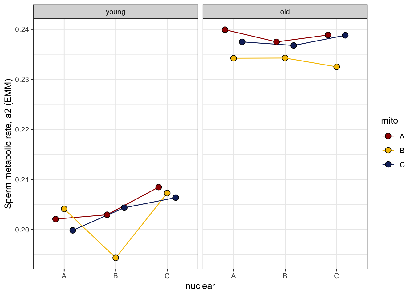

Past versions of unnamed-chunk-65-1.png

Version	Author	Date
a7bae31	MartinGarlovsky	2024-10-09

>>> Raw data and means

sperm_met_raw <- emmeans(met_mod_test, ~ mito * nuclear * age) %>% as_tibble() %>% 
  ggplot(aes(x = nuclear, y = emmean, fill = mito)) +
  geom_jitter(data = sperm_met,
              aes(y = p.a2, colour = mito),
               position = position_jitterdodge(dodge.width = .5, jitter.width = .1),
              size = 0.75, alpha = .1) +
  geom_jitter(data = sperm_met %>% 
                group_by(LINE, age) %>% 
                summarise(mn = mean(p.a2)) %>% 
                separate(LINE, into = c("mito", "nuclear", NA), sep = "(?<=.)", remove = FALSE),
              aes(y = mn, colour = mito),
              position = position_jitterdodge(dodge.width = .5, jitter.width = .1),
              alpha = .85, size = 2) +
  geom_errorbar(aes(ymin = lower.CL, ymax = upper.CL), 
                width = .25, position = position_dodge(width = .5)) +
  geom_point(size = 3, pch = 21, position = position_dodge(width = .5)) +
  labs(y = 'Sperm metabolic rate, a2 (EMM ± 95% CIs)') +
  scale_colour_manual(values = met3) +
  scale_fill_manual(values = met3) +
  coord_cartesian(ylim = c(0.14, 0.34)) +
  facet_wrap(~ age) +
  theme_bw() + 
  theme() + 
  ggrepel::geom_text_repel(data = sperm_met %>% filter(a2 > 50), aes(y = p.a2), label = "CA1, a2 = 0.55") + 
  geom_text(data = sperm_met %>% group_by(mito, nuclear, age) %>% count(), aes(y = 0.14, label = n), 
            size = 2, position = position_dodge(width = .5)) + 
  #ggsave('figures/sperm_met_raw.pdf', height = 4, width = 8, dpi = 600, useDingbats = FALSE) +
  NULL

sperm_met_raw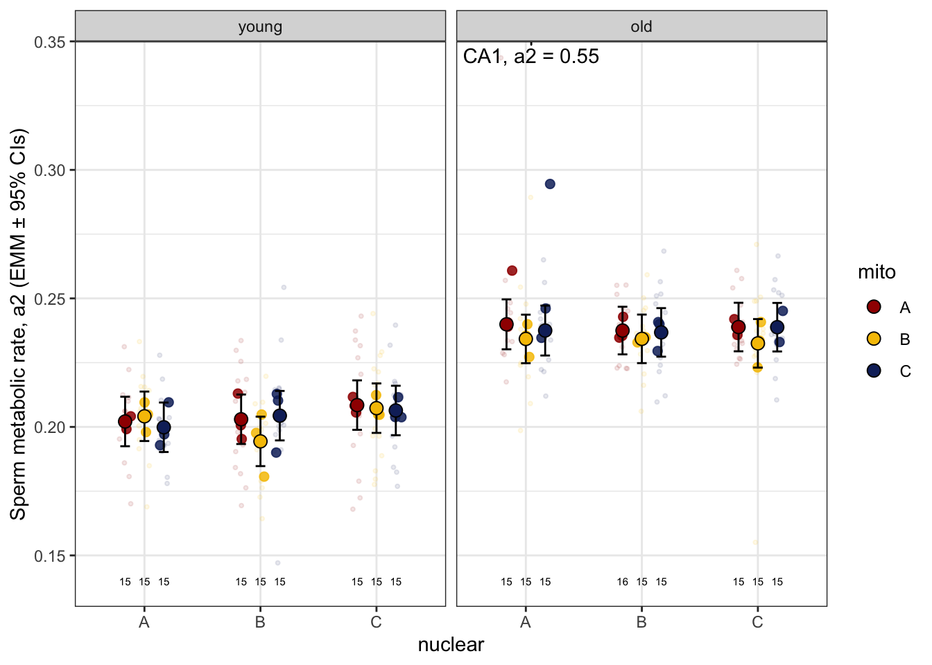

Past versions of unnamed-chunk-66-1.png

Version	Author	Date
0ffce9c	MartinGarlovsky	2024-10-10
a7bae31	MartinGarlovsky	2024-10-09

>>> Matched vs. mismatched

met_mod_coevo <- lmerTest::lmer(p.a2 ~ coevolved * age + (1 + age|LINE), 
                                data = sperm_met %>% filter(a2 <= 30), REML = TRUE)

anova(met_mod_coevo, type = "III", ddf = "Kenward-Roger")

Type III Analysis of Variance Table with Kenward-Roger's method
                Sum Sq  Mean Sq NumDF  DenDF  F value    Pr(>F)    
coevolved     0.000071 0.000071     1 25.163   0.2392    0.6290    
age           0.069532 0.069532     1 25.163 234.5554 2.905e-14 ***
coevolved:age 0.000364 0.000364     1 25.163   1.2289    0.2781    
---
Signif. codes:  0 '***' 0.001 '**' 0.01 '*' 0.05 '.' 0.1 ' ' 1

>>> Mito-type analysis

met_mod_outlier_rm_snp <- lmerTest::lmer(p.a2 ~ mito_snp * nuclear * age + (1 + age|LINE), 
                                         data = sperm_met %>% filter(a2 <= 30))

anova(met_mod_outlier_rm_snp, type = "III", ddf = "Kenward-Roger")

Type III Analysis of Variance Table with Kenward-Roger's method
                       Sum Sq  Mean Sq NumDF  DenDF  F value    Pr(>F)    
mito_snp             0.001854 0.000232     8 8.8749   0.7690    0.6392    
nuclear              0.001367 0.000683     2 8.8614   2.2672    0.1603    
age                  0.054751 0.054751     1 9.0178 181.6457 2.792e-07 ***
mito_snp:nuclear     0.002263 0.000323     7 8.8640   1.0724    0.4509    
mito_snp:age         0.001489 0.000186     8 8.8749   0.6175    0.7456    
nuclear:age          0.000634 0.000317     2 8.8614   1.0511    0.3894    
mito_snp:nuclear:age 0.001933 0.000276     7 8.8640   0.9162    0.5358    
---
Signif. codes:  0 '***' 0.001 '**' 0.01 '*' 0.05 '.' 0.1 ' ' 1

> Sperm competition

We measured sperm defence (P1) and offence (P2) for focal males against a competitor brown eyed (BW) male for 15 males from each mitonuclear population. The data shows overdispersion, so we use male ID as an observation level random effect. Note that here, we only measured young (5 day old) males.

>> Sperm defence (P1)

First we take a look at the data for each Day and Block, and see how P1 changes with copulation duration (cop.dur).

>>> Day and block effect

defence %>% 
  ggplot(aes(x = nuclear, y = P1, colour = mito)) +
  geom_jitter(position = position_jitterdodge(dodge.width = .65, jitter.width = .15),
              alpha = .5) +
  labs(y = 'Sperm viability (EMM ± 95% CIs)') +
  scale_colour_manual(values = met3) +
  scale_fill_manual(values = met3) +
  theme_bw() + 
  theme() + 
  stat_summary(position = position_dodge(width = 0.65)) +
  facet_grid(Day ~ Block) +
  NULL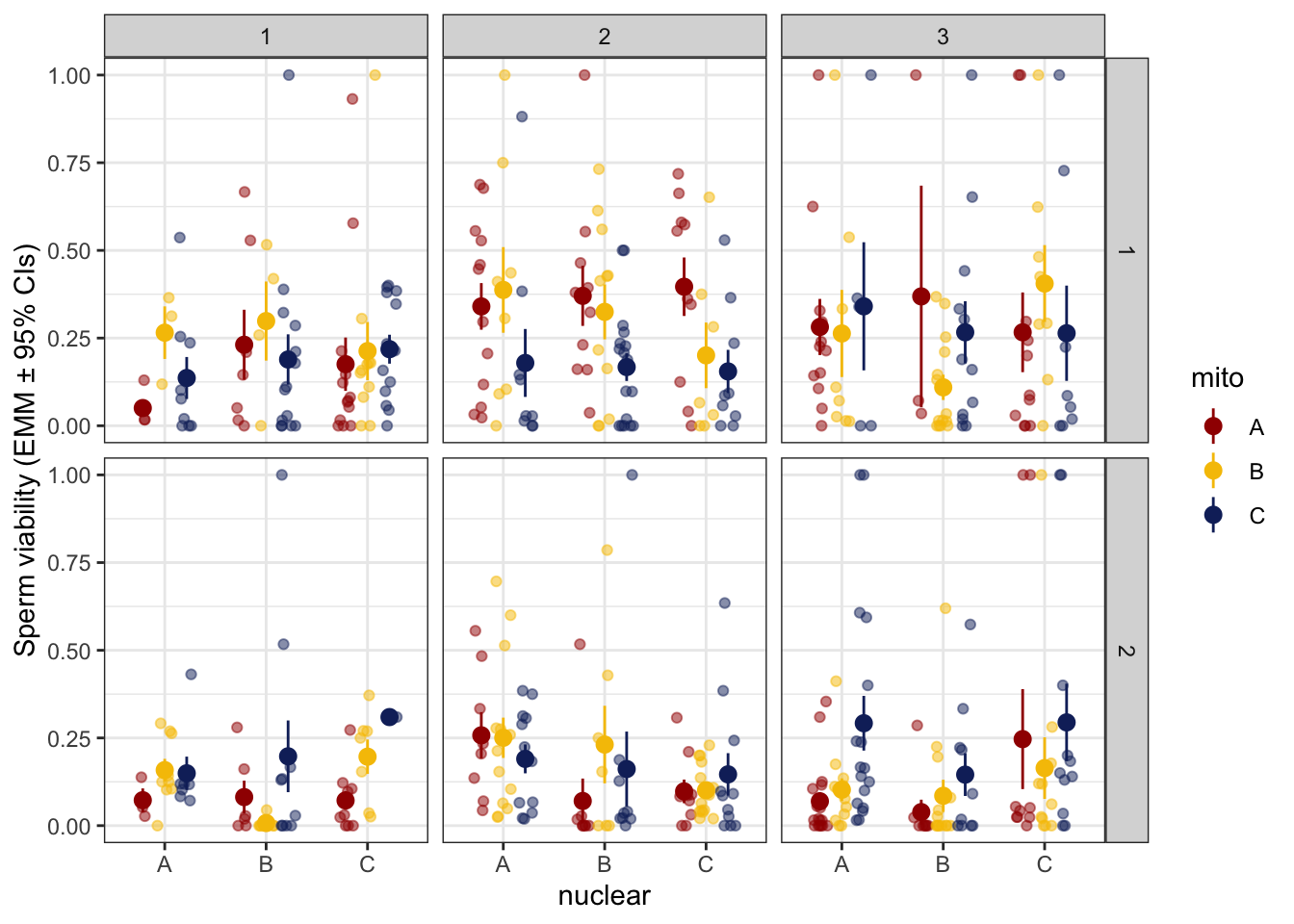

Past versions of unnamed-chunk-69-1.png

Version	Author	Date
0ffce9c	MartinGarlovsky	2024-10-10
a7bae31	MartinGarlovsky	2024-10-09

>>> Copulation duration

defence %>% 
  ggplot(aes(x = cop.dur, y = P1, colour = nuclear)) +
  geom_smooth(method = "lm", se = FALSE) +
  scale_colour_manual(values = met3) +
  scale_fill_manual(values = met3) +
  theme_bw() + 
  theme() + 
  facet_grid(Day ~ Block) +
  NULL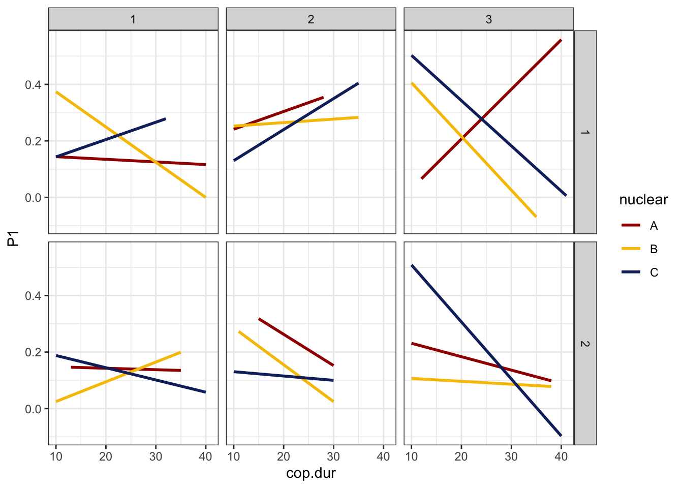

Past versions of unnamed-chunk-70-1.png

Version	Author	Date
a7bae31	MartinGarlovsky	2024-10-09

p1.mod1 <- glmer(cbind(RED, BW) ~ mito * nuclear + Day + cop.dur + (1 + cop.dur|LINE) + (1|ID) + (1|Block),
                 data = defence, family = binomial, 
                 control= glmerControl(optimizer="bobyqa", optCtrl=list(maxfun=50000))
                 )

>>> Check diagnostics

performance::check_model(p1.mod1)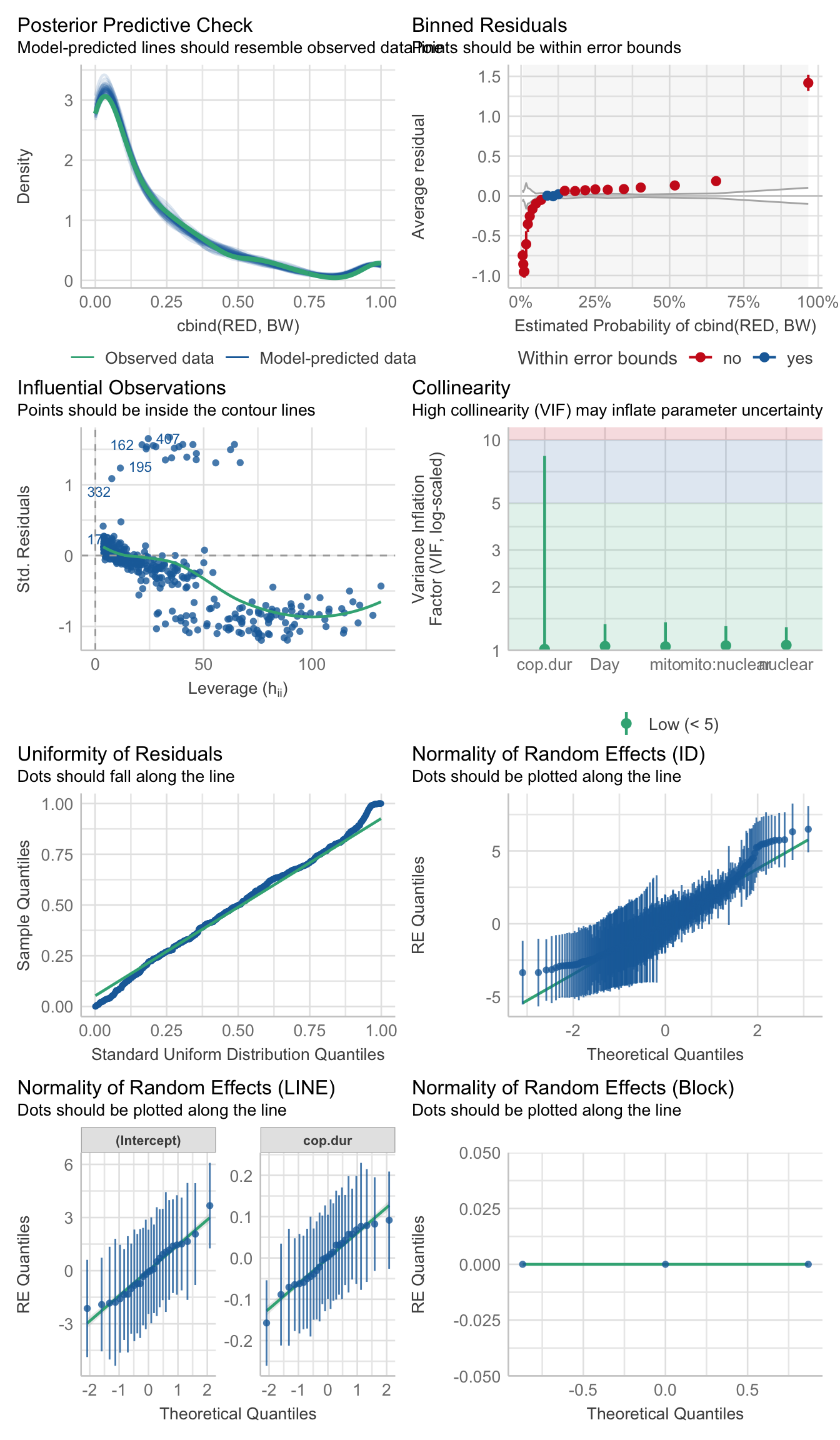

Past versions of unnamed-chunk-72-1.png

Version	Author	Date
0ffce9c	MartinGarlovsky	2024-10-10
a7bae31	MartinGarlovsky	2024-10-09

performance::check_overdispersion(p1.mod1)

# Overdispersion test

 dispersion ratio = 0.887
          p-value = 0.224

testDispersion(p1.mod1)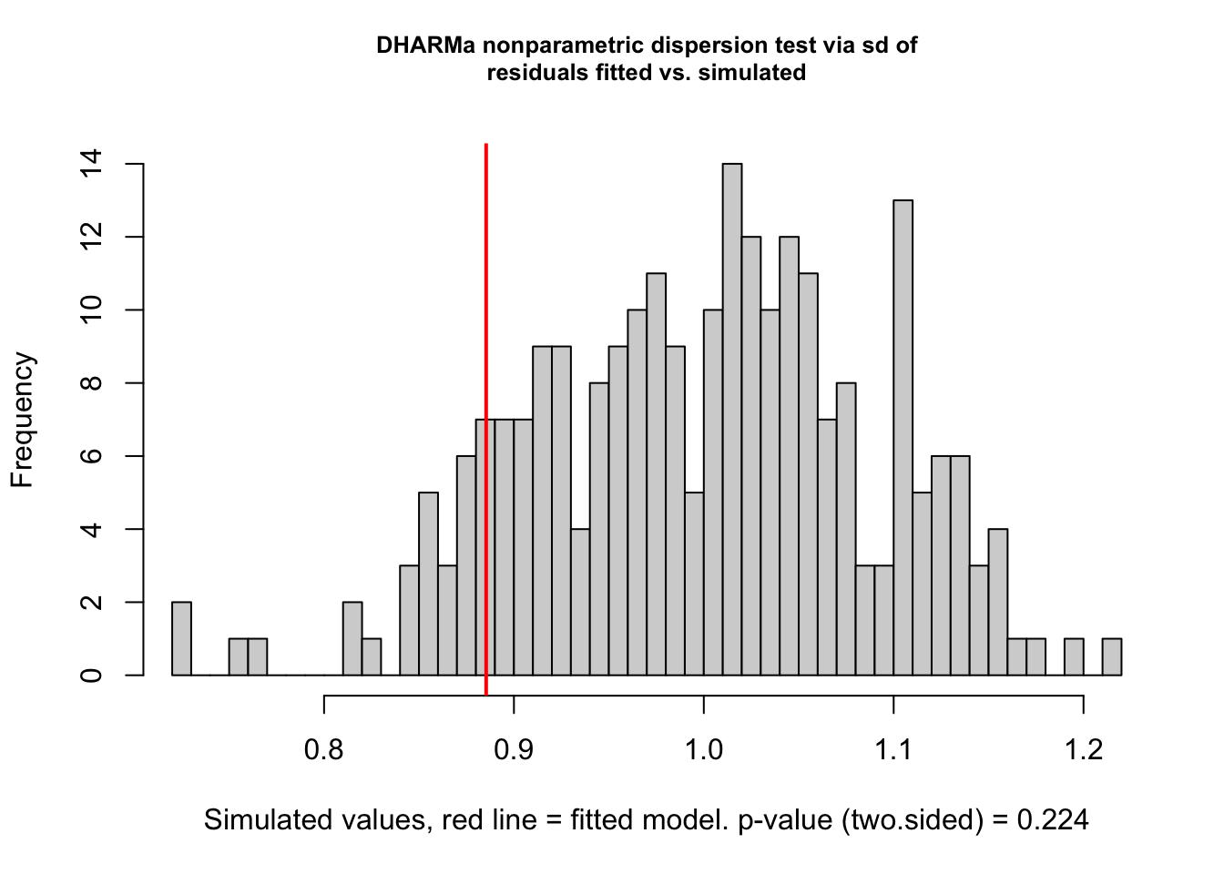

Past versions of unnamed-chunk-73-1.png

Version	Author	Date
a7bae31	MartinGarlovsky	2024-10-09

    DHARMa nonparametric dispersion test via sd of residuals fitted vs.
    simulated

data:  simulationOutput
dispersion = 0.8871, p-value = 0.224
alternative hypothesis: two.sided

simulationOutput <- simulateResiduals(fittedModel = p1.mod1, plot = FALSE)
hist(residuals(simulationOutput))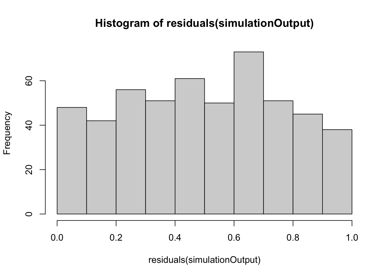

Past versions of unnamed-chunk-73-2.png

Version	Author	Date
a7bae31	MartinGarlovsky	2024-10-09

hist(residuals(simulationOutput, quantileFunction = qnorm, outlierValues = c(-7,7)))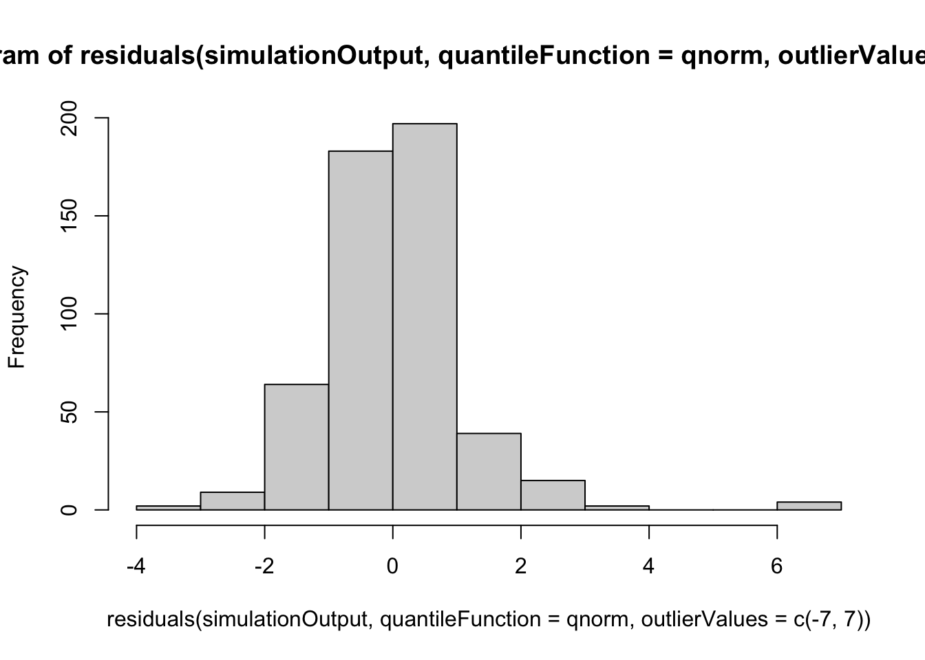

Past versions of unnamed-chunk-73-3.png

Version	Author	Date
a7bae31	MartinGarlovsky	2024-10-09

plot(simulationOutput)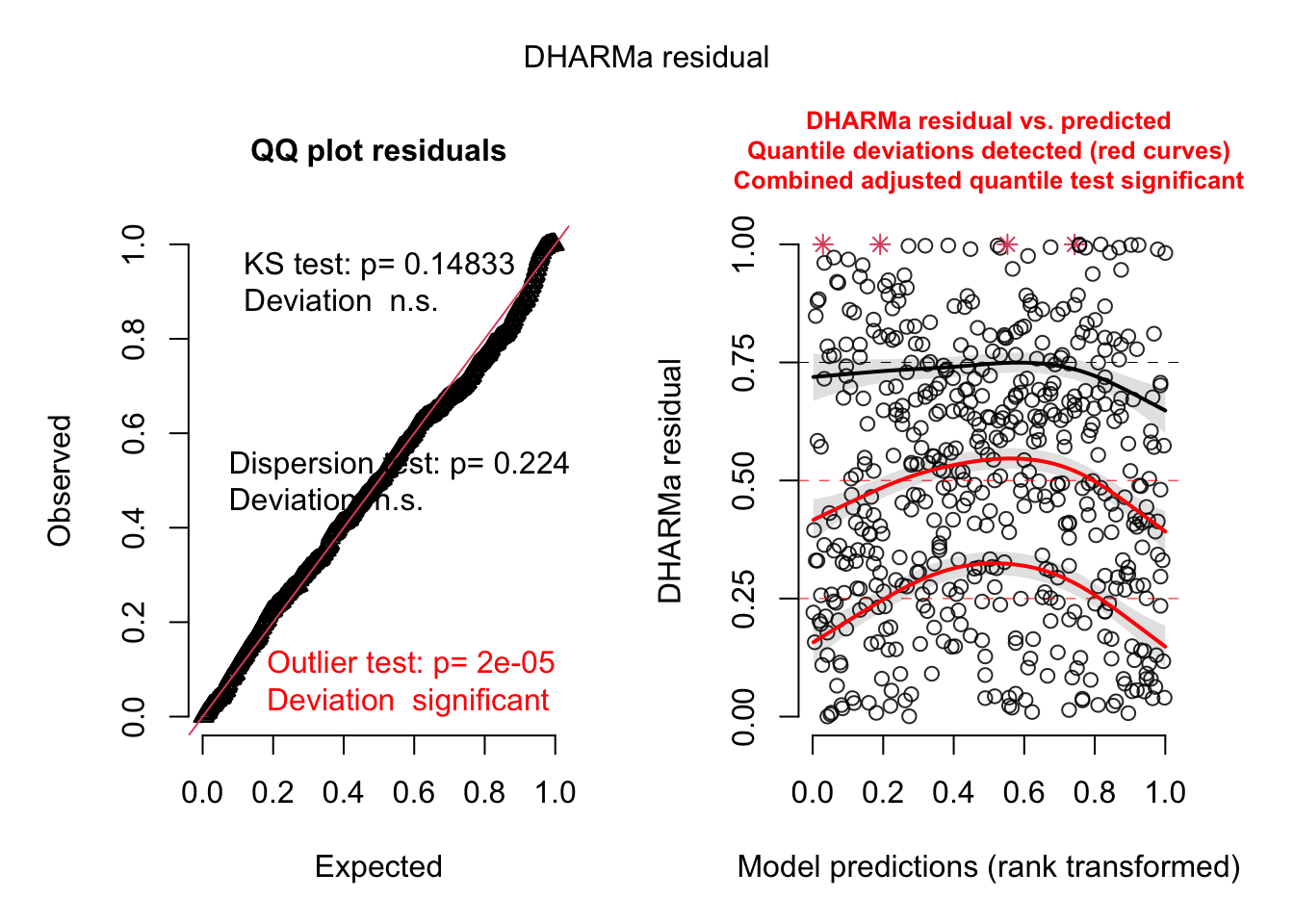

Past versions of unnamed-chunk-73-4.png

Version	Author	Date
a7bae31	MartinGarlovsky	2024-10-09

>>> Results

car::Anova(p1.mod1, type = "3") %>% 
  broom::tidy() %>% 
  as_tibble() %>% #write_csv("output/anova_tables/male_P1.csv") %>% # save anova table for supp. tables
  kable(digits = 3, 
        caption = 'Analysis of Deviance Table (Type III Wald chisquare tests)') %>% 
  kable_styling(full_width = FALSE)

Analysis of Deviance Table (Type III Wald chisquare tests)

term	statistic	df	p.value
(Intercept)	6.279	1	0.012
mito	0.574	2	0.751
nuclear	12.795	2	0.002
Day	16.861	1	0.000
cop.dur	2.209	1	0.137
mito:nuclear	2.455	4	0.653

# posthoc tests
bind_rows(emmeans(p1.mod1, pairwise ~ nuclear, adjust = "tukey")$contrasts %>% broom::tidy() %>%
            rename(p.value = adj.p.value),
          emmeans(p1.mod1, pairwise ~ Day, adjust = "tukey")$contrasts %>% broom::tidy()) %>% 
  mutate(p.val = ifelse(p.value < 0.001, '< 0.001', round(p.value, 3))) %>% 
  select(-p.value, -term) %>% 
  kable(digits = 3, 
        caption = 'Posthoc Tukey tests to compare which groups differ') %>% 
  kable_styling(full_width = FALSE) %>%
  kableExtra::group_rows("Nuclear", 1, 3) %>%
  kableExtra::group_rows("Day", 4, 4)

Posthoc Tukey tests to compare which groups differ

contrast	null.value	estimate	std.error	df	statistic	p.val
Nuclear
A - B	0	0.954	0.272	Inf	3.510	0.001
A - C	0	0.291	0.260	Inf	1.118	0.503
B - C	0	-0.663	0.269	Inf	-2.466	0.036
Day
Day1 - Day2	0	0.886	0.216	Inf	4.106	< 0.001

p1plot_raw <- emmeans(p1.mod1, ~ mito * nuclear, type = 'response') %>% as_tibble() %>% 
  ggplot(aes(x = nuclear, y = prob, fill = mito)) +
  geom_jitter(data = defence,
              aes(y = P1, colour = mito),
               position = position_jitterdodge(dodge.width = .5, jitter.width = .1),
              alpha = .25) + 
  geom_jitter(data = defence %>% 
                group_by(LINE) %>% 
                summarise(mn = mean(P1)) %>% 
                separate(LINE, into = c("mito", "nuclear", NA), sep = "(?<=.)", remove = FALSE),
              aes(y = mn, colour = mito),
              position = position_jitterdodge(dodge.width = .5, jitter.width = .1),
              alpha = .85, size = 2) +
  geom_errorbar(aes(ymin = asymp.LCL, ymax = asymp.UCL), 
                width = .25, position = position_dodge(width = .5)) +
  geom_point(size = 3, pch = 21, position = position_dodge(width = .5)) +
  labs(y = expression(P[1]*" (EMM ± 95% CIs)")) +
  scale_colour_manual(values = met3) +
  scale_fill_manual(values = met3) +
  theme_bw() + 
  theme() + 
  geom_text(data = defence %>% 
              group_by(mito, nuclear) %>% count(), aes(y = -0.04, label = n), 
            size = 2, position = position_dodge(width = .5)) + 
  #ggsave('figures/p1plot_raw.pdf', height = 4, width = 5, dpi = 600, useDingbats = FALSE) +
  NULL

p1plot_raw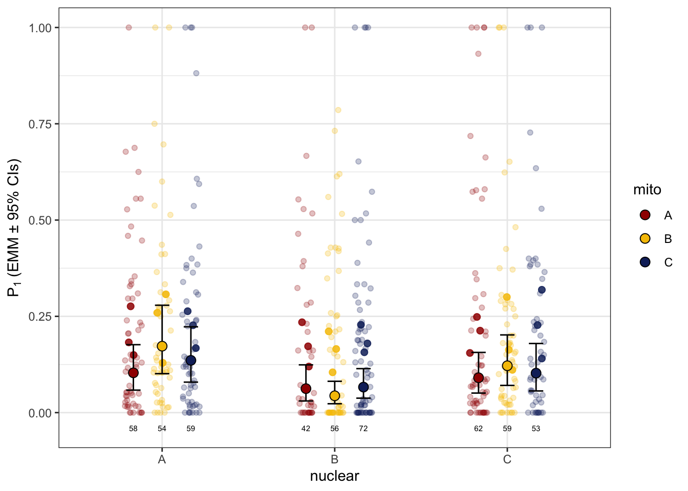

Past versions of unnamed-chunk-74-1.png

Version	Author	Date
a7bae31	MartinGarlovsky	2024-10-09

>>> Matched vs. mismatched

p1.coevo <- glmer(cbind(RED, BW) ~ coevolved + Day + cop.dur + (1 + cop.dur|LINE) + (1|ID) + (1|Block),
                 data = defence, family = binomial, 
                 control= glmerControl(optimizer="bobyqa", optCtrl=list(maxfun=50000))
                 )

car::Anova(p1.coevo, type = "3")

Analysis of Deviance Table (Type III Wald chisquare tests)

Response: cbind(RED, BW)
              Chisq Df Pr(>Chisq)    
(Intercept)  7.2827  1  0.0069623 ** 
coevolved    1.8058  1  0.1790107    
Day         13.4235  1  0.0002485 ***
cop.dur      1.8764  1  0.1707460    
---
Signif. codes:  0 '***' 0.001 '**' 0.01 '*' 0.05 '.' 0.1 ' ' 1

>>> Mito-type analysis

p1.snp <- glmer(cbind(RED, BW) ~ mito_snp * nuclear + Day + cop.dur + (1 + cop.dur|LINE) + (1|ID) + (1|Block),
                 data = defence, family = binomial, 
                 control= glmerControl(optimizer="bobyqa", optCtrl=list(maxfun=1e6)))

car::Anova(p1.snp, type = "3")

Analysis of Deviance Table (Type III Wald chisquare tests)

Response: cbind(RED, BW)
                   Chisq Df Pr(>Chisq)    
(Intercept)       8.0205  1   0.004625 ** 
mito_snp          4.9541  8   0.762472    
nuclear           0.0089  2   0.995559    
Day              15.2078  1  9.631e-05 ***
cop.dur           2.0267  1   0.154558    
mito_snp:nuclear  8.6698  7   0.277241    
---
Signif. codes:  0 '***' 0.001 '**' 0.01 '*' 0.05 '.' 0.1 ' ' 1

>> Sperm offence (P2)

>>> Check covariates

>>>> Day and block effect

offence %>% 
  ggplot(aes(x = nuclear, y = P2, colour = mito)) +
  geom_jitter(position = position_jitterdodge(dodge.width = .65, jitter.width = .15),
              alpha = .5) +
  labs(y = 'Sperm viability (EMM ± 95% CIs)') +
  scale_colour_manual(values = met3) +
  scale_fill_manual(values = met3) +
  theme_bw() + 
  theme() + 
  stat_summary(position = position_dodge(width = 0.65)) +
  facet_grid(Day ~ Block) +
  NULL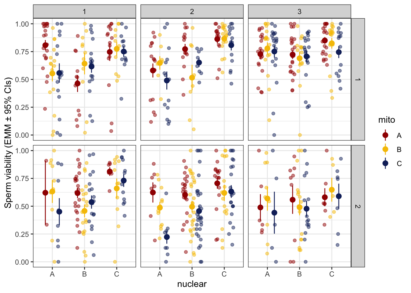

Past versions of unnamed-chunk-77-1.png

Version	Author	Date
a7bae31	MartinGarlovsky	2024-10-09

>>>> Copulation duration

offence %>% 
  ggplot(aes(x = cop.dur, y = P2, colour = nuclear)) +
  geom_smooth(method = "lm", se = FALSE) +
  scale_colour_manual(values = met3) +
  scale_fill_manual(values = met3) +
  theme_bw() + 
  theme() + 
  facet_grid(Day ~ Block) +
  NULL

Past versions of unnamed-chunk-78-1.png

Version	Author	Date
a7bae31	MartinGarlovsky	2024-10-09

>>>

p2.mod1 <- glmer(cbind(RED, BW) ~ mito * nuclear + Day + cop.dur + (1 + cop.dur|LINE) + (1|ID) + (1|Block),
                 data = offence, family = binomial)

>>>> Check diagnostics

performance::check_model(p2.mod1)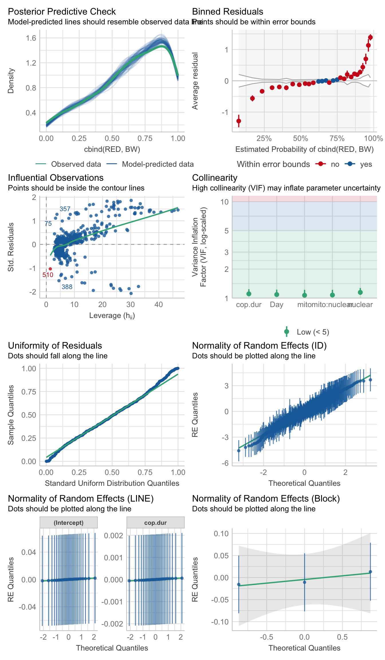

Past versions of unnamed-chunk-80-1.png

Version	Author	Date
0ffce9c	MartinGarlovsky	2024-10-10
a7bae31	MartinGarlovsky	2024-10-09

performance::check_overdispersion(p2.mod1)

# Overdispersion test

 dispersion ratio =   1.085
          p-value = < 0.001

testDispersion(p2.mod1)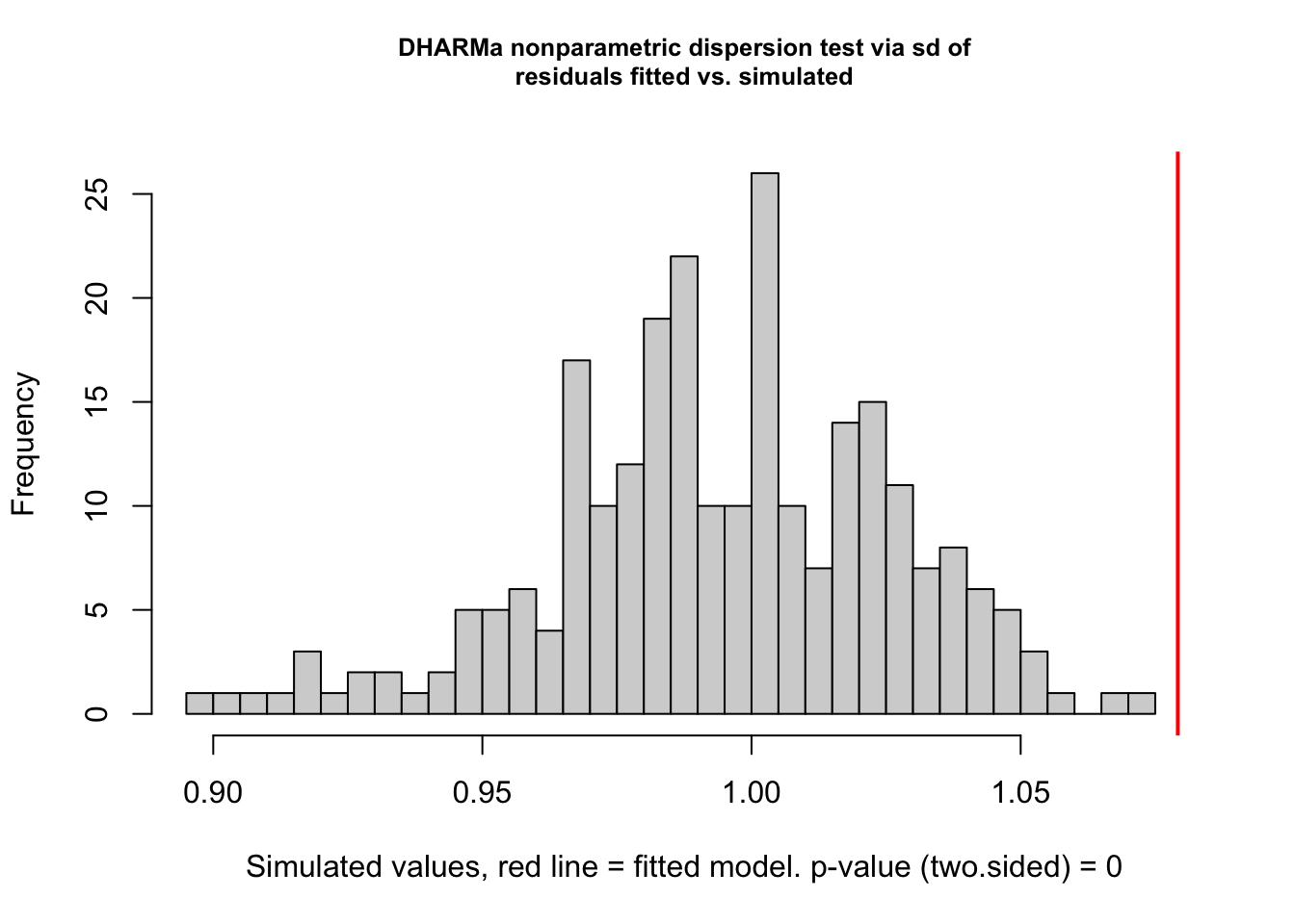

Past versions of unnamed-chunk-81-1.png

Version	Author	Date
a7bae31	MartinGarlovsky	2024-10-09

    DHARMa nonparametric dispersion test via sd of residuals fitted vs.
    simulated

data:  simulationOutput
dispersion = 1.0853, p-value < 2.2e-16
alternative hypothesis: two.sided

simulationOutput <- simulateResiduals(fittedModel = p2.mod1, plot = FALSE)
hist(residuals(simulationOutput))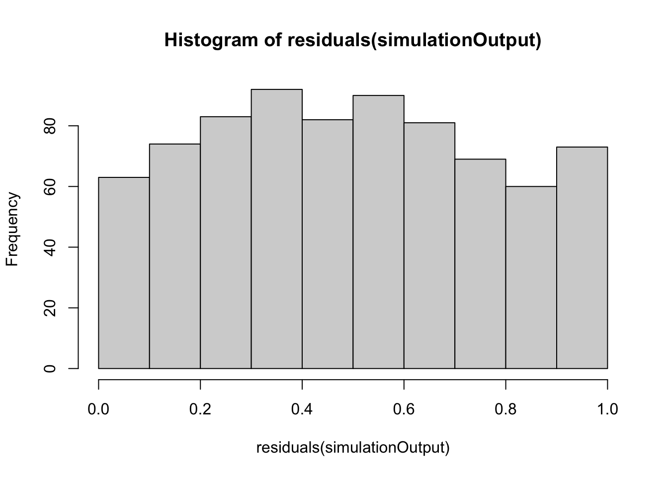

Past versions of unnamed-chunk-81-2.png

Version	Author	Date
a7bae31	MartinGarlovsky	2024-10-09

hist(residuals(simulationOutput, quantileFunction = qnorm, outlierValues = c(-7,7)))

Past versions of unnamed-chunk-81-3.png

Version	Author	Date
a7bae31	MartinGarlovsky	2024-10-09

plot(simulationOutput)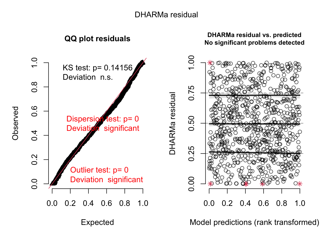

Past versions of unnamed-chunk-81-4.png

Version	Author	Date
a7bae31	MartinGarlovsky	2024-10-09

car::Anova(p2.mod1, type = "3") %>% 
  broom::tidy() %>% 
  as_tibble() %>% #write_csv("output/anova_tables/male_P2.csv") %>% # save anova table for supp. tables
  kable(digits = 3, 
        caption = 'Analysis of Deviance Table (Type III Wald chisquare tests)') %>% 
  kable_styling(full_width = FALSE)

Analysis of Deviance Table (Type III Wald chisquare tests)

term	statistic	df	p.value
(Intercept)	12.529	1	0.000
mito	10.657	2	0.005
nuclear	54.549	2	0.000
Day	49.924	1	0.000
cop.dur	0.000	1	0.988
mito:nuclear	3.681	4	0.451

# posthoc tests
bind_rows(emmeans(p2.mod1, pairwise ~ mito, adjust = "tukey")$contrasts %>% broom::tidy() %>%
            rename(p.value = adj.p.value),
          emmeans(p2.mod1, pairwise ~ nuclear, adjust = "tukey")$contrasts %>% broom::tidy() %>%
            rename(p.value = adj.p.value),
          emmeans(p2.mod1, pairwise ~ Day, adjust = "tukey")$contrasts %>% broom::tidy()) %>% 
  mutate(p.val = ifelse(p.value < 0.001, '< 0.001', round(p.value, 3))) %>% 
  select(-p.value, -term) %>% 
  kable(digits = 3, 
        caption = 'Posthoc Tukey tests to compare which groups differ') %>% 
  kable_styling(full_width = FALSE) %>%
  kableExtra::group_rows("Mitochondria", 1, 3) %>%
  kableExtra::group_rows("Nuclear", 4, 6) %>%
  kableExtra::group_rows("Day", 7, 7)

Posthoc Tukey tests to compare which groups differ

contrast	null.value	estimate	std.error	df	statistic	p.val
Mitochondria
A - B	0	0.250	0.141	Inf	1.777	0.177
A - C	0	0.455	0.140	Inf	3.260	0.003
B - C	0	0.205	0.140	Inf	1.458	0.311
Nuclear
A - B	0	0.027	0.143	Inf	0.191	0.98
A - C	0	-0.921	0.149	Inf	-6.157	< 0.001
B - C	0	-0.948	0.142	Inf	-6.689	< 0.001
Day
Day1 - Day2	0	0.875	0.124	Inf	7.066	< 0.001

p2plot_raw <- emmeans(p2.mod1, ~ mito * nuclear, type = 'response') %>% as_tibble() %>% 
  ggplot(aes(x = nuclear, y = prob, fill = mito)) +
  geom_jitter(data = offence,
              aes(y = P2, colour = mito),
               position = position_jitterdodge(dodge.width = .5, jitter.width = .1),
              alpha = .25) + 
  geom_jitter(data = offence %>% 
                group_by(LINE) %>% 
                summarise(mn = mean(P2)) %>% 
                separate(LINE, into = c("mito", "nuclear", NA), sep = "(?<=.)", remove = FALSE),
              aes(y = mn, colour = mito),
              position = position_jitterdodge(dodge.width = .5, jitter.width = .1),
              alpha = .85, size = 2) +
  geom_errorbar(aes(ymin = asymp.LCL, ymax = asymp.UCL), 
                width = .25, position = position_dodge(width = .5)) +
  geom_point(size = 3, pch = 21, position = position_dodge(width = .5)) +
  labs(y = expression(P[2]*" (EMM ± 95% CIs)")) +
  scale_colour_manual(values = met3) +
  scale_fill_manual(values = met3) +
  theme_bw() + 
  theme() + 
  geom_text(data = defence %>% 
              group_by(mito, nuclear) %>% count(), aes(y = -0.04, label = n), 
            size = 2, position = position_dodge(width = .5)) + 
  #ggsave('figures/p1plot_raw.pdf', height = 4, width = 5, dpi = 600, useDingbats = FALSE) +
  NULL

p2plot_raw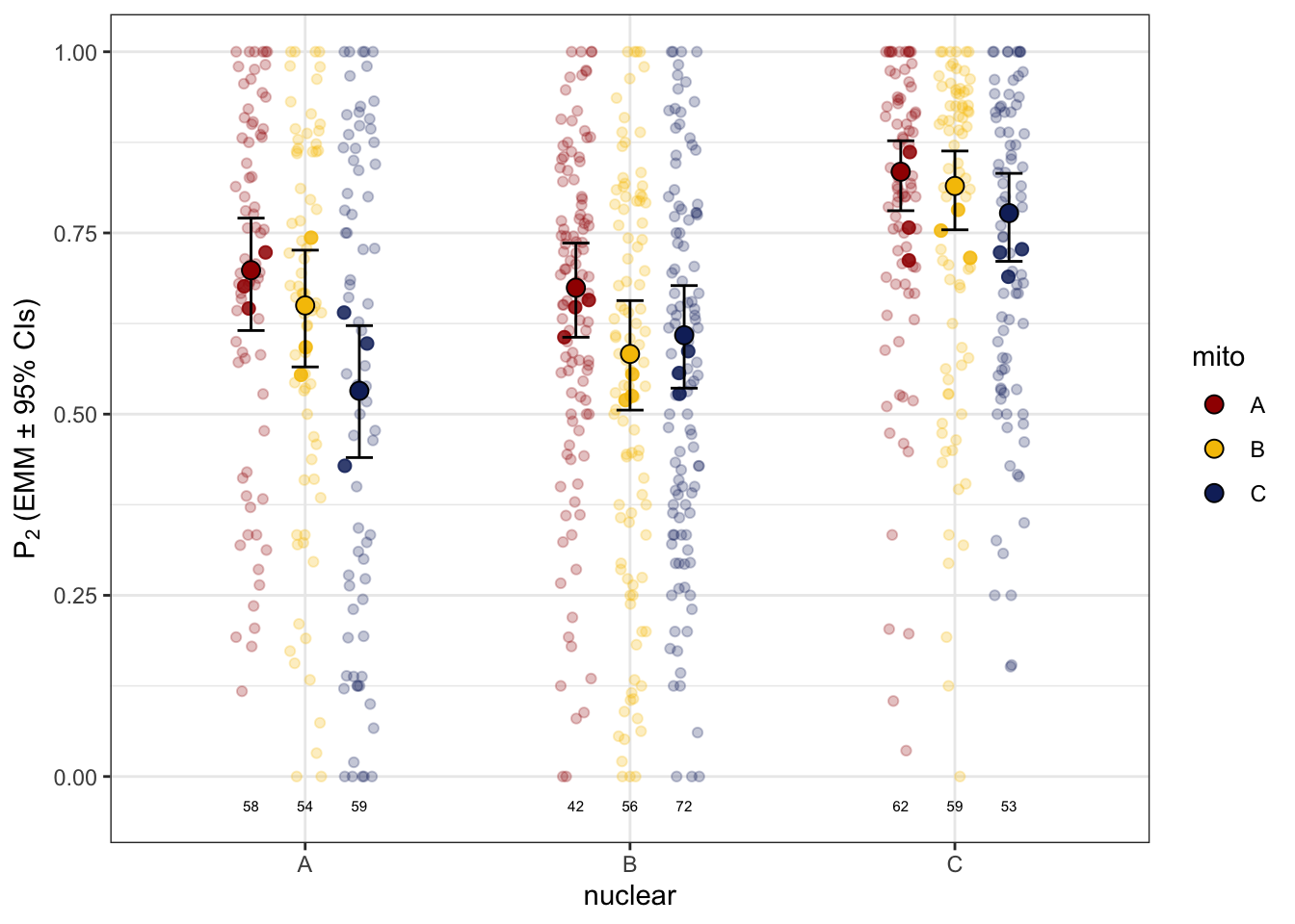

Past versions of unnamed-chunk-83-1.png

Version	Author	Date
a7bae31	MartinGarlovsky	2024-10-09

>>> Matched vs. mismatched

p2.coevo <- glmer(cbind(RED, BW) ~ coevolved + Day + cop.dur + (1|LINE) + (1|ID) + (1|Block),
                 data = offence, family = binomial, 
                 control= glmerControl(optimizer="bobyqa", optCtrl=list(maxfun=50000)))

car::Anova(p2.coevo, type = "3")

Analysis of Deviance Table (Type III Wald chisquare tests)

Response: cbind(RED, BW)
              Chisq Df Pr(>Chisq)    
(Intercept) 13.5083  1  0.0002375 ***
coevolved    0.0543  1  0.8157506    
Day         51.4143  1  7.479e-13 ***
cop.dur      0.2653  1  0.6064804    
---
Signif. codes:  0 '***' 0.001 '**' 0.01 '*' 0.05 '.' 0.1 ' ' 1

>>> Mito-type analysis

p2.snp <- glmer(cbind(RED, BW) ~ mito_snp * nuclear + Day + cop.dur + (1 + cop.dur|LINE) + (1|ID) + (1|Block),
                 data = offence, family = binomial)

car::Anova(p2.snp, type = "3")

Analysis of Deviance Table (Type III Wald chisquare tests)

Response: cbind(RED, BW)
                   Chisq Df Pr(>Chisq)    
(Intercept)       3.0321  1    0.08163 .  
mito_snp         10.0480  8    0.26167    
nuclear           8.1189  2    0.01726 *  
Day              44.6794  1  2.321e-11 ***
cop.dur           0.0209  1    0.88510    
mito_snp:nuclear  3.8621  7    0.79551    
---
Signif. codes:  0 '***' 0.001 '**' 0.01 '*' 0.05 '.' 0.1 ' ' 1

Combined plot

comb_spermcomp <- bind_rows(
  emmeans(p1.mod1, ~ mito * nuclear, type = 'response') %>% as_tibble() %>% mutate(trt = "P1"),
  emmeans(p2.mod1, ~ mito * nuclear, type = 'response') %>% as_tibble() %>% mutate(trt = "P2")) %>% 
  ggplot(aes(x = nuclear, y = prob, fill = mito)) +
  geom_line(aes(group = mito, colour = mito), position = position_dodge(width = .5)) +
  geom_point(size = 3, pch = 21, position = position_dodge(width = .5)) +
  labs(y = 'Proportion sired (EMM)') +
  scale_colour_manual(values = met3) +
  scale_fill_manual(values = met3) +
  facet_wrap(~trt) +
  theme_bw() + 
  theme() +
  NULL

comb_spermcomp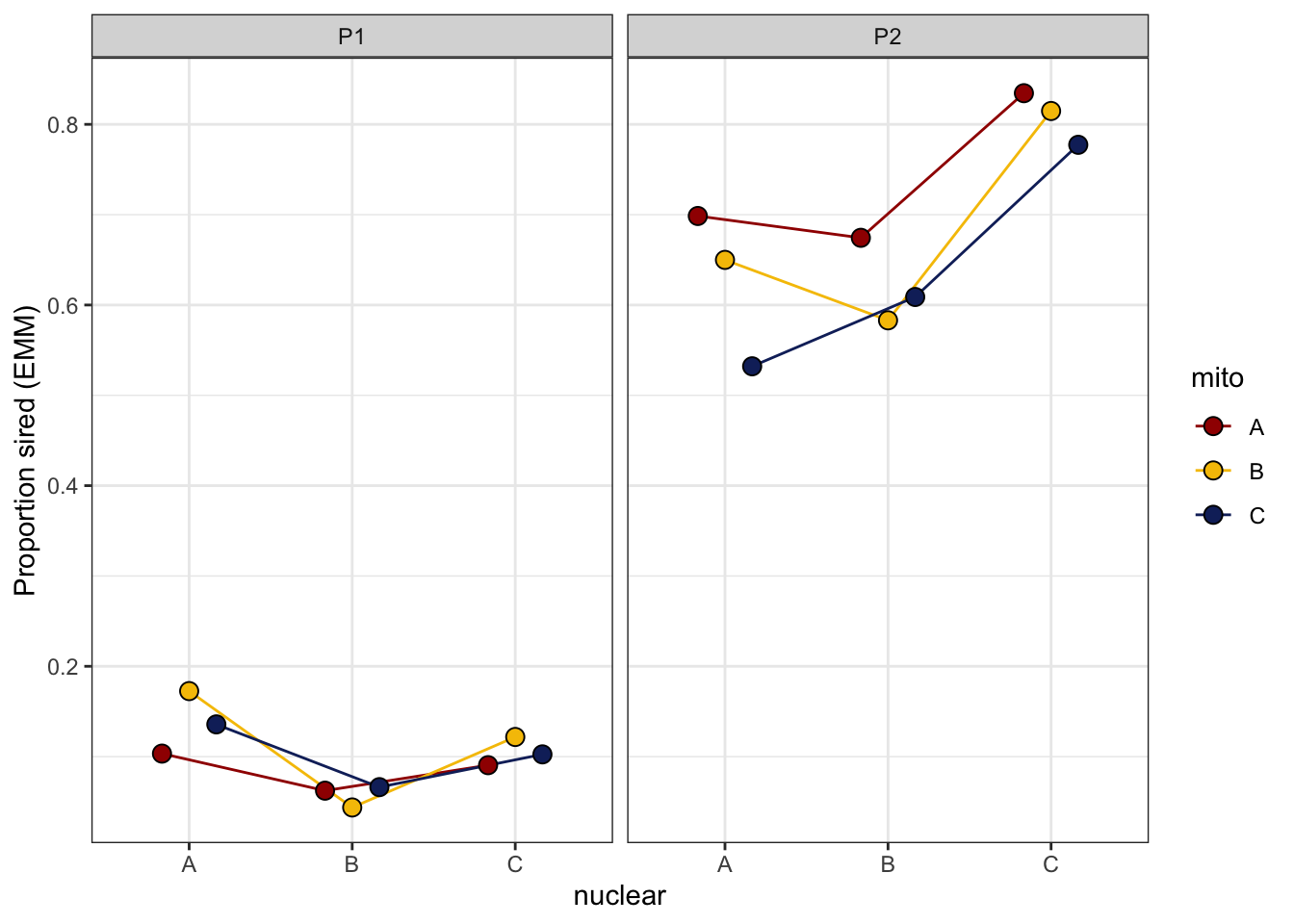

Past versions of unnamed-chunk-86-1.png

Version	Author	Date
a7bae31	MartinGarlovsky	2024-10-09

>> Correlation of P1 vs P2

Finally, we tested whether there was a correlation between P1 and P2 using the model estimated marginal means for each genotype. We can visualise this either as the ranked means (1-9) or as a scatterplot.

pdat <- bind_rows(emmeans(p1.mod1, ~ mito * nuclear) %>% as_tibble() %>% mutate(met = "P1"),
                  emmeans(p2.mod1, ~ mito * nuclear) %>% as_tibble() %>% mutate(met = "P2")) %>% 
  mutate(mt = rep(1:9, 2))

>>> Ranked means

pdat %>% 
  group_by(met) %>% 
  mutate(rank = dense_rank(desc(emmean))) %>% 
  ggplot(aes(x = met, y = rank)) +
  geom_point(size = 5, aes(shape = mito, colour = nuclear)) +
  geom_line(aes(group = mt)) +
  scale_colour_manual(values = met3) +
  scale_fill_manual(values = met3) +
  scale_y_continuous(breaks = 1:9) +
  theme_bw()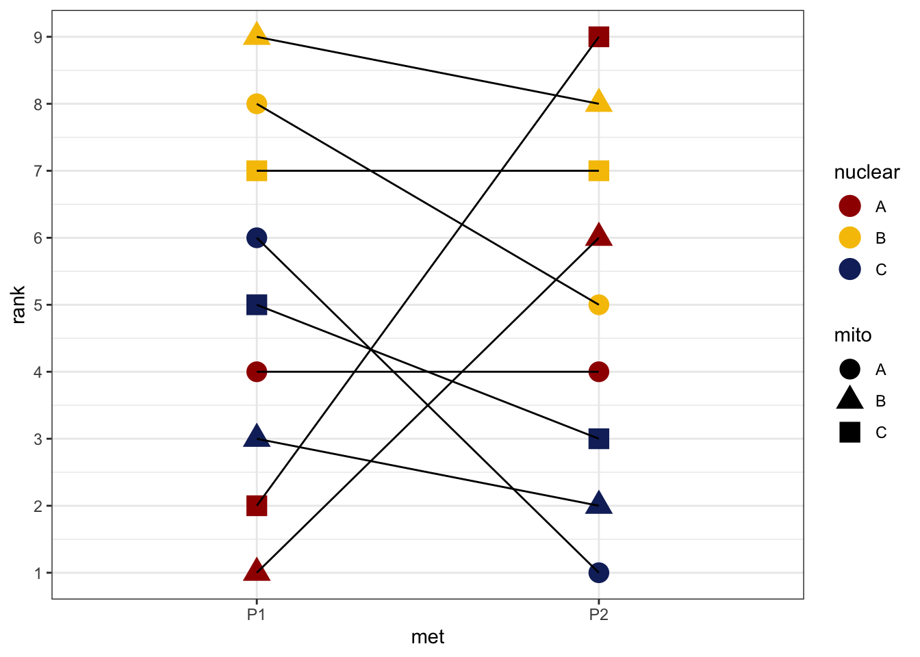

Past versions of unnamed-chunk-88-1.png

Version	Author	Date
a7bae31	MartinGarlovsky	2024-10-09

>>> Scatterplot

pdat.wide <- pdat %>% select(mito, nuclear, emmean, mt, met) %>% 
  pivot_wider(names_from = met, values_from = emmean)

pdat.wide %>% 
  ggplot(aes(x = P1, y = P2)) +
  geom_point(size = 5, aes(shape = mito, colour = nuclear)) +
  ggpubr::stat_cor(method = "s") +
  #geom_smooth(method = "lm", lty = 2, se = FALSE) +
  labs(x = "logit(P1)", y = "logit(P2)") +
  scale_colour_manual(values = met3) +
  scale_fill_manual(values = met3) +
  theme_bw() +
  theme() +
  #ggsave('figures/sperm_comp_cor.pdf', height = 4, width = 4.8, dpi = 600, useDingbats = FALSE) +
  NULL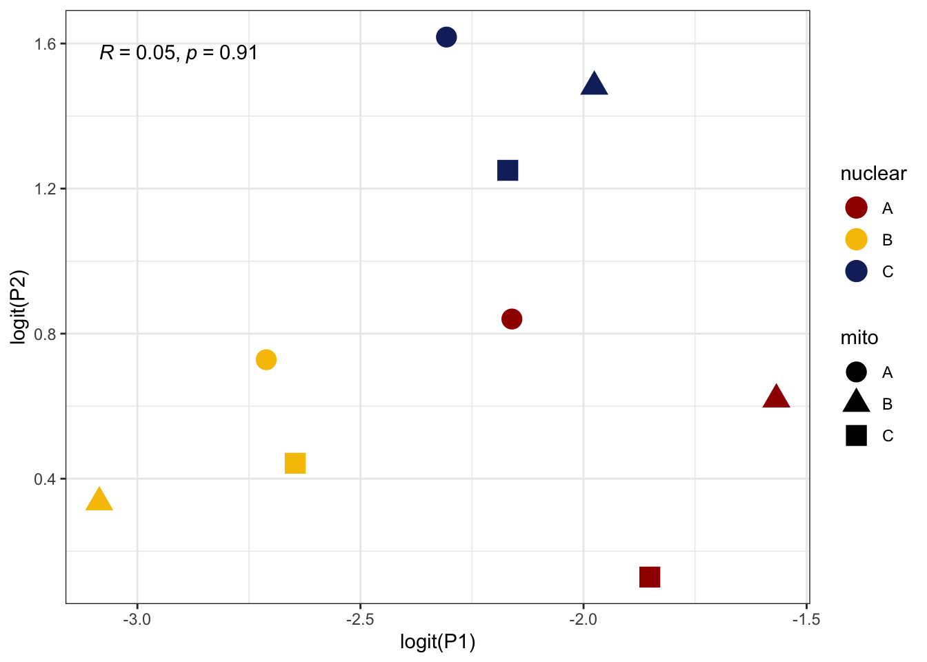

Past versions of unnamed-chunk-89-1.png

Version	Author	Date
a7bae31	MartinGarlovsky	2024-10-09

cor.test(pdat.wide$P1, pdat.wide$P2, method = "s")

    Spearman's rank correlation rho

data:  pdat.wide$P1 and pdat.wide$P2
S = 114, p-value = 0.9116
alternative hypothesis: true rho is not equal to 0
sample estimates:
 rho 
0.05 

Session information

sessionInfo()

R version 4.4.0 (2024-04-24)
Platform: aarch64-apple-darwin20
Running under: macOS Sonoma 14.6.1

Matrix products: default
BLAS:   /Library/Frameworks/R.framework/Versions/4.4-arm64/Resources/lib/libRblas.0.dylib 
LAPACK: /Library/Frameworks/R.framework/Versions/4.4-arm64/Resources/lib/libRlapack.dylib;  LAPACK version 3.12.0

locale:
[1] en_US.UTF-8/en_US.UTF-8/en_US.UTF-8/C/en_US.UTF-8/en_US.UTF-8

time zone: Europe/London
tzcode source: internal

attached base packages:
[1] stats     graphics  grDevices utils     datasets  methods   base     

other attached packages:
 [1] conflicted_1.2.0 showtext_0.9-7   showtextdb_3.0   sysfonts_0.8.9  
 [5] knitrhooks_0.0.4 knitr_1.48       kableExtra_1.4.0 emmeans_1.10.5  
 [9] DHARMa_0.4.7     lme4_1.1-35.5    Matrix_1.7-1     lubridate_1.9.3 
[13] forcats_1.0.0    stringr_1.5.1    dplyr_1.1.4      purrr_1.0.2     
[17] readr_2.1.5      tidyr_1.3.1      tibble_3.2.1     ggplot2_3.5.1   
[21] tidyverse_2.0.0  workflowr_1.7.1 

loaded via a namespace (and not attached):
  [1] Rdpack_2.6.1        rlang_1.1.4         magrittr_2.0.3     
  [4] git2r_0.35.0        compiler_4.4.0      getPass_0.2-4      
  [7] mgcv_1.9-1          systemfonts_1.1.0   callr_3.7.6        
 [10] vctrs_0.6.5         pkgconfig_2.0.3     fastmap_1.2.0      
 [13] backports_1.5.0     MetBrewer_0.2.0     labeling_0.4.3     
 [16] utf8_1.2.4          promises_1.3.0      rmarkdown_2.28     
 [19] tzdb_0.4.0          ps_1.8.1            nloptr_2.1.1       
 [22] xfun_0.48           cachem_1.1.0        jsonlite_1.8.9     
 [25] highr_0.11          later_1.3.2         broom_1.0.7        
 [28] parallel_4.4.0      R6_2.5.1            gap.datasets_0.0.6 
 [31] qgam_1.3.4          bslib_0.8.0         stringi_1.8.4      
 [34] car_3.1-3           boot_1.3-31         jquerylib_0.1.4    
 [37] numDeriv_2016.8-1.1 estimability_1.5.1  iterators_1.0.14   
 [40] Rcpp_1.0.13         httpuv_1.6.15       splines_4.4.0      
 [43] timechange_0.3.0    tidyselect_1.2.1    abind_1.4-8        
 [46] rstudioapi_0.17.1   yaml_2.3.10         codetools_0.2-20   
 [49] doParallel_1.0.17   processx_3.8.4      plyr_1.8.9         
 [52] lattice_0.22-6      lmerTest_3.1-3      shiny_1.9.1        
 [55] bayestestR_0.15.0   withr_3.0.2         coda_0.19-4.1      
 [58] evaluate_1.0.1      xml2_1.3.6          ggpubr_0.6.0       
 [61] pillar_1.9.0        carData_3.0-5       gap_1.6            
 [64] whisker_0.4.1       foreach_1.5.2       insight_1.0.1      
 [67] generics_0.1.3      rprojroot_2.0.4     hms_1.1.3          
 [70] munsell_0.5.1       scales_1.3.0        minqa_1.2.8        
 [73] xtable_1.8-4        glue_1.8.0          tools_4.4.0        
 [76] see_0.9.0           ggsignif_0.6.4      fs_1.6.5           
 [79] mvtnorm_1.3-1       grid_4.4.0          rbibutils_2.3      
 [82] datawizard_1.0.0    colorspace_2.1-1    nlme_3.1-166       
 [85] patchwork_1.3.0     performance_0.13.0  Formula_1.2-5      
 [88] cli_3.6.3           fansi_1.0.6         viridisLite_0.4.2  
 [91] svglite_2.1.3       gtable_0.3.6        rstatix_0.7.2      
 [94] sass_0.4.9          digest_0.6.37       pbkrtest_0.5.3     
 [97] ggrepel_0.9.6       farver_2.1.2        memoise_2.0.1      
[100] htmltools_0.5.8.1   lifecycle_1.0.4     httr_1.4.7         
[103] mime_0.12           MASS_7.3-61